In this article I will show how to build Tensorflow Lite based jelly bears classifier using Arduino Nano 33 BLE Sense.
Before you will continue reading please watch short introduction:
Currently a machine learning solution can be deployed not only on very powerful machines containing GPU cards but also on a really small devices. Of course such a devices has a some limitation eg. memory etc. To deploy ML model we need to prepare it. The Tensorflow framework allows you to convert neural networks to Tensorflow Lite which can be installed on the edge devices eg. Arduino Nano.
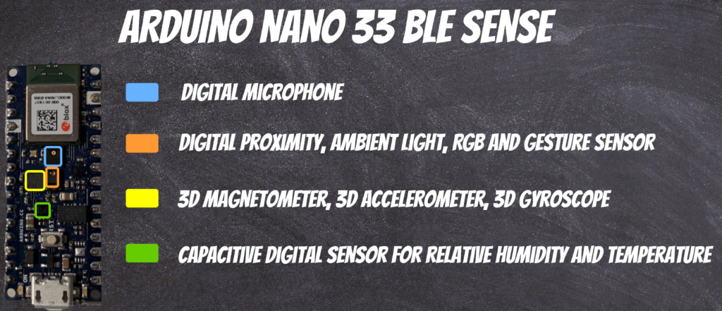
Arduino Nano 33 BLE Sense is equipped with many sensors that allow for the implementation of many projects eg.:
Digital microphone
Digital proximity, ambient light, RGB and gesture sensor
3D magnetometer, 3D accelerometer, 3D gyroscope
Capacitive digital sensor for relative humidity and temperature
Examples which I have used in this project can be found here.
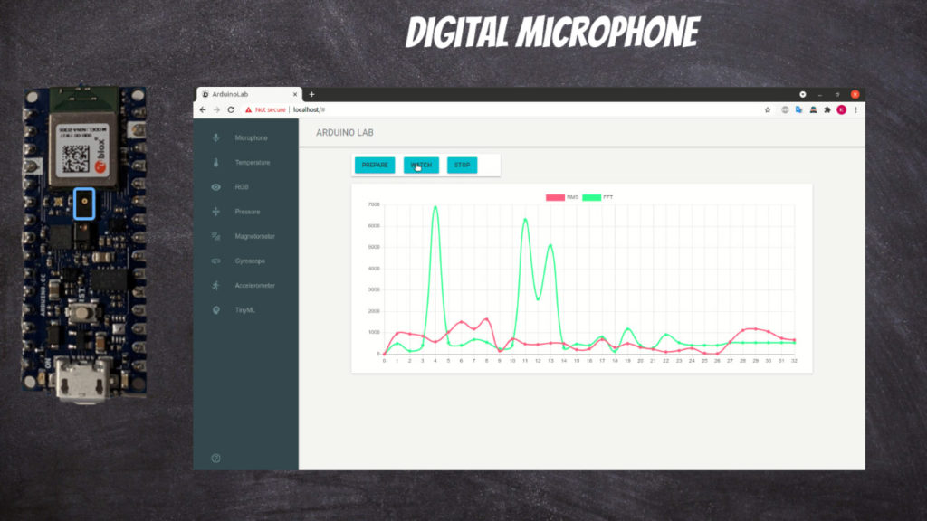
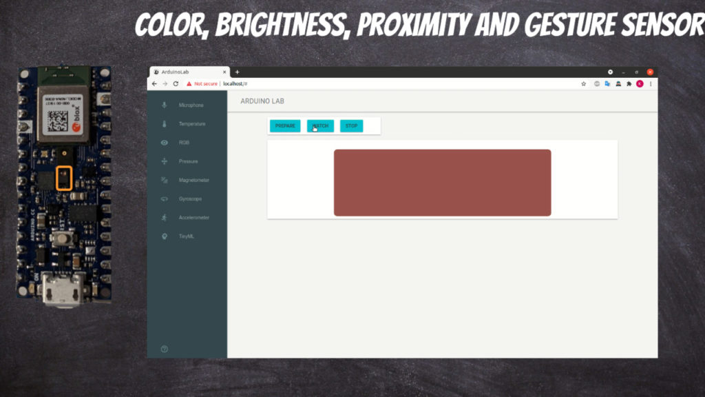
To simplify device usage I have build Arduino Lab project where you can test and investigate listed sensors directly on the web browser.
The project dependencies are packed into docker image to simplify usage.
Before you start the project you will need to connect Arduino through USB (the Arduino will communicate with docker container through /dev/ttyACM0)
git clone https://github.com/qooba/tinyml-arduino.git
cd tinyml-arduino
./run.server.sh
# in another terminal tab
./run.nginx.sh
# go inside server container
docker exec -it arduino /bin/bash
./start.sh
For each sensor type you can click Prepare button which will build and deploy appropriate Arduino code.
NOTE:
Sometimes you will have to deploy to arduino manually to do this you will need to
go to arduino container
docker exec -it arduino /bin/bash
cd /arduino
make rgb
Here you have complete Makefile with all types of implemented sensors.
You can start observations using Watch button.
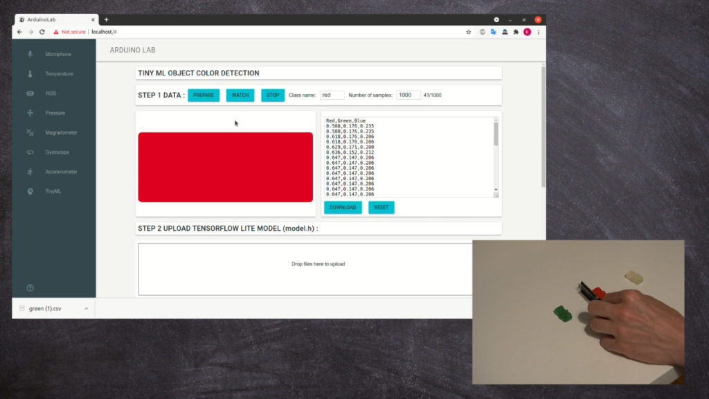
Now we will build TinyML solution.
In the first step we will capture training data:
The training data will be saved in the csv format. You will need to repeat the proces for each class you will detect.
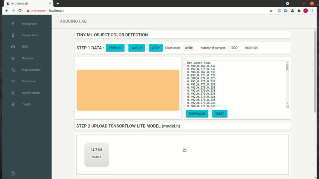
Captured data will be uploaded to the Colab Notebook.
Here I fully base on the project Fruit identification using Arduino and TensorFlow.
In the notebook we train the model using Tensorflow then convert it to Tensorflow Lite and finally encode to hex format (model.h header file) which is readable by Arduino.
Now we compile and upload model.h header file using drag and drop mechanism.
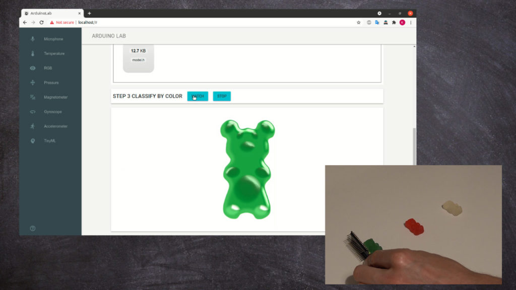
Finally we can classify the jelly bears by the color:
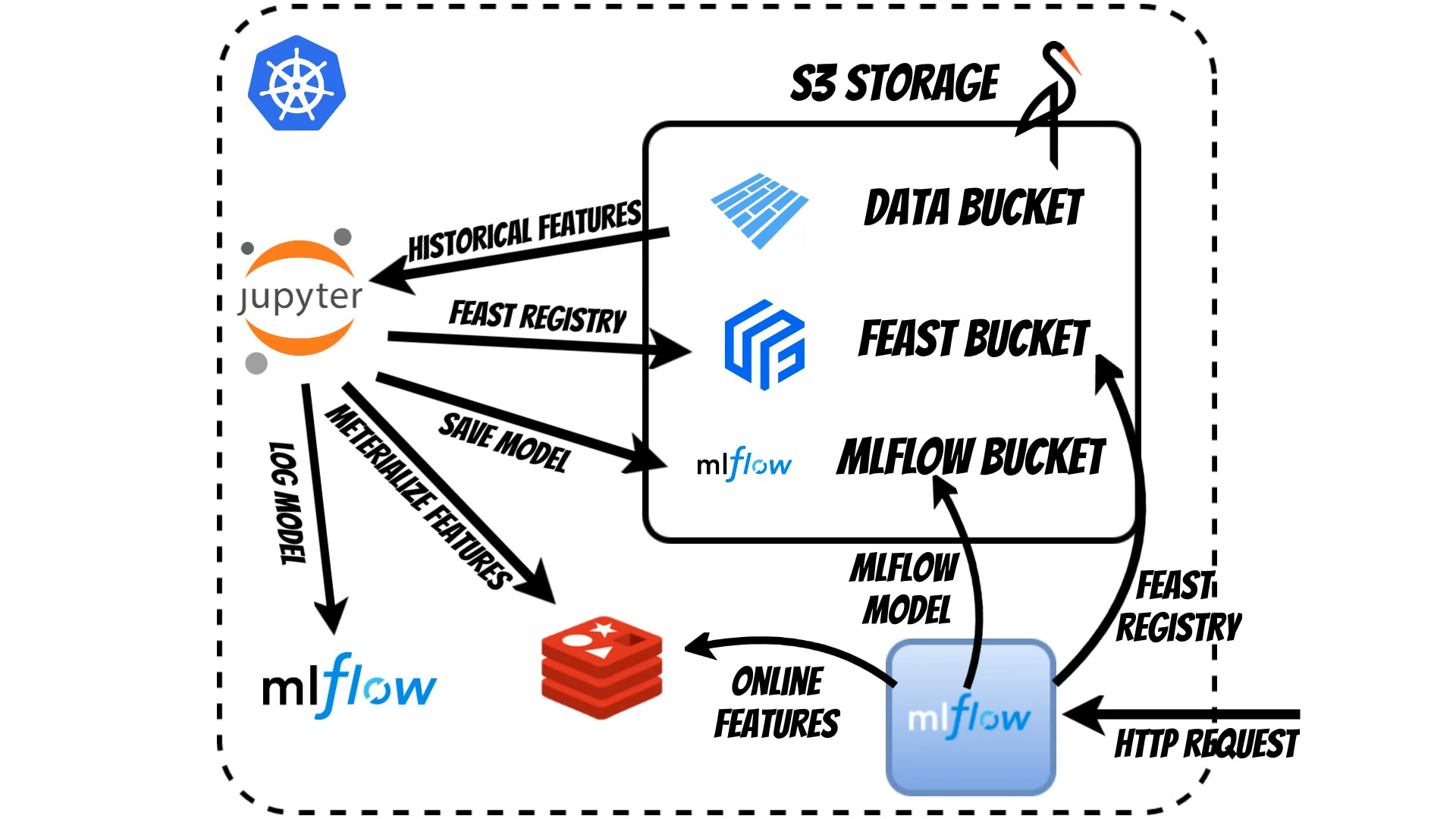
To better visualize the whole process we will use the Propensity to buy example where I base on the Kaggle examples and data.
We start in Jupyter Notebook where we prepare Feast feature store schema which is kept in S3.
We can simply inspect the Feast schema in Jupyter Notebook:
from feast import FeatureStore
from IPython.core.display import display, HTML
import json
from json2html import *
import warnings
warnings.filterwarnings('ignore')

class FeastSchema:
    def __init__(self, repo_path: str):
        self.store = FeatureStore(repo_path=repo_path)

    def show_schema(self, skip_meta: bool= False):
        feast_schema=self.__project_show_schema(skip_meta)
        display(HTML(json2html.convert(json = feast_schema)))

    def show_table_schema(self, table: str, skip_meta: bool= False):
        feasture_tables_dictionary=self.__project_show_schema(skip_meta)
        display(HTML(json2html.convert(json = {table:feasture_tables_dictionary[table]})))

    def __project_show_schema(self, skip_meta: bool= False):
        entities_dictionary={}
        feast_entities=self.store.list_entities()
        for entity in feast_entities:
            entity_dictionary=entity.to_dict()
            entity_spec=entity_dictionary['spec']
            entities_dictionary[entity_spec['name']]=entity_spec

        feasture_tables_dictionary={}
        feast_feature_tables=self.store.list_feature_views()
        for feature_table in feast_feature_tables:
            feature_table_dict=json.loads(str(feature_table))
            feature_table_spec=feature_table_dict['spec']
            feature_table_name=feature_table_spec['name']
            feature_table_spec.pop('name',None)
            if 'entities' in feature_table_spec:
                feature_table_entities=[]
                for entity in feature_table_spec['entities']:
                    feature_table_entities.append(entities_dictionary[entity])
                feature_table_spec['entities']=feature_table_entities

            if not skip_meta:
                feature_table_spec['meta']=feature_table_dict['meta']
            else:
                feature_table_spec.pop('input',None)
                feature_table_spec.pop('ttl',None)
                feature_table_spec.pop('online',None)

            feasture_tables_dictionary[feature_table_name]=feature_table_spec

        return feasture_tables_dictionary


FeastSchema(".").show_schema()
#FeastSchema(".").show_schema(skip_meta=True)
#FeastSchema(".").show_table_schema('driver_hourly_stats')
#FeastSchema().show_tables()
In our case we store the data in Apache Parquet files in S3 bucket.
Using the Feast we can fetch the historical features and train the model using Scikit-learn library
Using MLflow we can simply deploy model as a microservice in k8s.
In our case we want to deploy the model models:/propensity_model/Production
which is currently assigned for Production. During start the MLflow will automatically fetch the proper model from S3:
In this article I will show how to process streams with Apache Flink and MLflow model
Before you will continue reading please watch short introduction:
Apache Flink allows for an efficient and scalable way of processing streams. It is a distributed processing engine which supports multiple sources like: Kafka, NiFi and many others
(if we need custom, we can create them ourselves).
Apache Flink also provides the framework for defining streams operations in languages like:
Java, Scala, Python and SQL.
To simplify the such definitions we can use Jupyter Notebook as a interface. Of course we can write in Python using PyFlink library but we can make it even easier using writing jupyter notebook extension (“magic words”).
Using Flink extension (magic.ipynb) we can simply use Flink SQL sql syntax directly in Jupyter Notebook.
To use the extesnions we need to load it:
%reload_ext flinkmagic
Then we need to initialize the Flink StreamEnvironment:
%flink_init_stream_env
Now we can use the SQL code for example:
FileSystem connector:
%%flink_execute_sql
CREATE TABLE MySinkTable (
    word varchar,
    cnt bigint) WITH (
        'connector.type' = 'filesystem',
        'format.type' = 'csv',
        'connector.path' = '/opt/flink/notebooks/data/word_count_output1')
The magic keyword will automatically execute SQL in existing StreamingEnvironment.
Now we can apply the Machine Learning model. In plain Flink we can use UDF function defined
in python but we will use MLflow model which wraps the ML frameworks (like PyTorch, Tensorflow, Scikit-learn etc.). Because MLflow expose homogeneous interface we can
create another “jupyter magic” which will automatically load MLflow model as a Flink function.
%%flink_sql_query
SELECT word as smstext, SPAM_CLASSIFIER(word) as smstype FROM MySourceKafkaTable
which in our case will fetch kafka events and classify it using MLflow spam classifier. The
results will be displayed in the realtime in the Jupyter Notebook as a events DataFrame.
If we want we can simply use other python libraries (like matplotlib and others) to create
graphical representation of the results eg. pie chart.
You can also use docker image: qooba/flink:dev to test and run notebooks inside.
Please check the run.sh
where you have all components (Kafka, MySQL, Jupyter with Flink, MLflow repository).
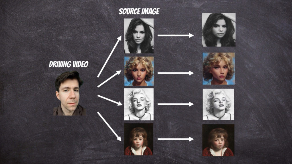
In this article I will show how to use artificial intelligence to add motion to the images and photos.
Before you will continue reading please watch short introduction:
Face reenactment
To bring photos to life we can use the face reenactment algorithm designed to transfer the facial movements in the video to another image.
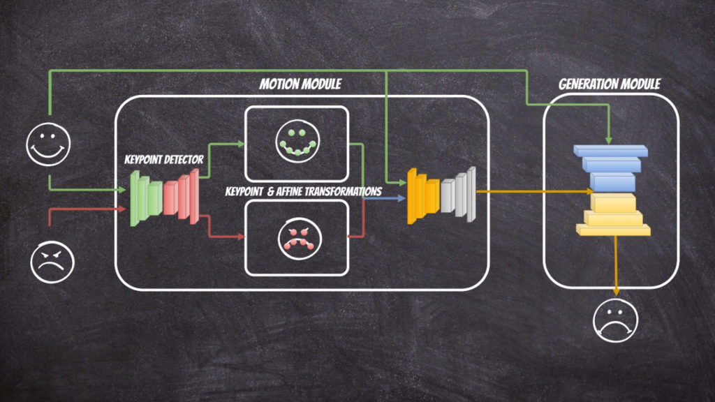
In this project I have used github implementation: https://github.com/AliaksandrSiarohin/first-order-model. Where the extensive description of the neural network architecture can be found in this paper. The solution contains of two parts: motion module and generation module.
The motion module at the first stage extracts the key points from the source and target image. In fact in the solution we assume that reference image which we can to the source and target image exists and at the first stage the transformations from reference image to source ([latex]T_{S \leftarrow R} (p_k)[/latex]) and target ([latex]T_{T \leftarrow R} (p_k)[/latex]) image is calculated respectively. Then the first order Taylor expansions [latex]\frac{d}{dp}T_{S \leftarrow R} (p)| {p=p_k}[/latex] and [latex]\frac{d}{dp}T_{T \leftarrow R} (p)| {p=p_k}[/latex] is used to calculate dense motion field.
The generation module use calculated dense motion field and source image to generate new image that will resemble target image.
The whole solution is packed into docker image thus we can simply reproduce the results using command:
NOTE: additional volumes (torch_models and checkpoints) are mount because during first run the trained neural networks are downloaded.
To reproduce the results we need to provide two files motion video and source image. In above example I put them into test directory and mount it into docker container (-v $(pwd)/test:/ai/test) to use them into it.
Below you have all command line options:
usage: prepare.py [-h] [--config CONFIG] [--checkpoint CHECKPOINT]
                  [--source_image SOURCE_IMAGE]
                  [--driving_video DRIVING_VIDEO] [--crop_image]
                  [--crop_image_padding CROP_IMAGE_PADDING [CROP_IMAGE_PADDING ...]]
                  [--crop_video] [--output OUTPUT] [--relative]
                  [--no-relative] [--adapt_scale] [--no-adapt_scale]
                  [--find_best_frame] [--best_frame BEST_FRAME] [--cpu]

first-order-model

optional arguments:
  -h, --help            show this help message and exit
  --config CONFIG       path to config
  --checkpoint CHECKPOINT
                        path to checkpoint to restore
  --source_image SOURCE_IMAGE
                        source image
  --driving_video DRIVING_VIDEO
                        driving video
  --crop_image, -ci     autocrop image
  --crop_image_padding CROP_IMAGE_PADDING [CROP_IMAGE_PADDING ...], -cip CROP_IMAGE_PADDING [CROP_IMAGE_PADDING ...]
                        autocrop image paddings left, upper, right, lower
  --crop_video, -cv     autocrop video
  --output OUTPUT       output video
  --relative            use relative or absolute keypoint coordinates
  --no-relative         don't use relative or absolute keypoint coordinates
  --adapt_scale         adapt movement scale based on convex hull of keypoints
  --no-adapt_scale      no adapt movement scale based on convex hull of
                        keypoints
  --find_best_frame     Generate from the frame that is the most alligned with
                        source. (Only for faces, requires face_aligment lib)
  --best_frame BEST_FRAME
                        Set frame to start from.
  --cpu                 cpu mode.
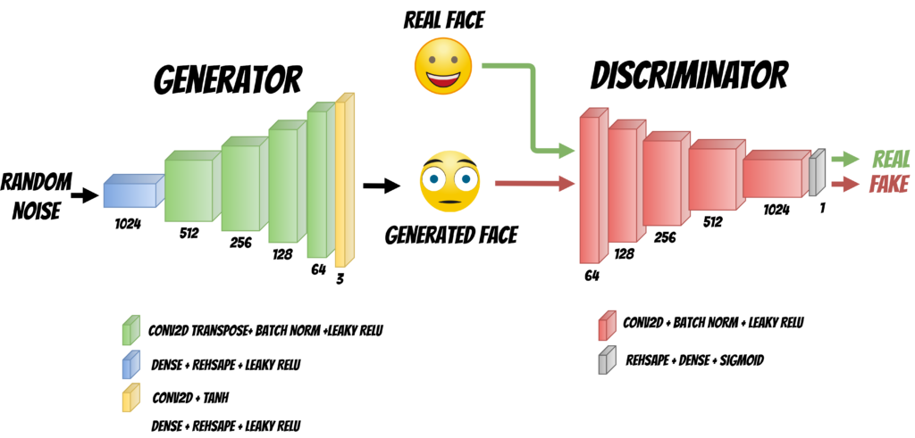
The GaN network consists of two parts of the Generator whose task is to generate the image from random input and a discriminator that checks if the generated image is realistic.
During training, the networks compete with each other, the generator tries to generate better and better images
and thereby deceive the Discriminator. On the other hand, the Discriminator learns to distinguish between real and generated photos.
To train the discriminator, we use both real photos and those generated by the generator.
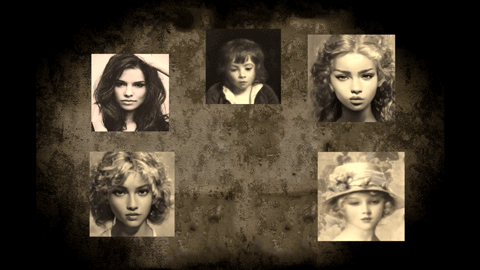
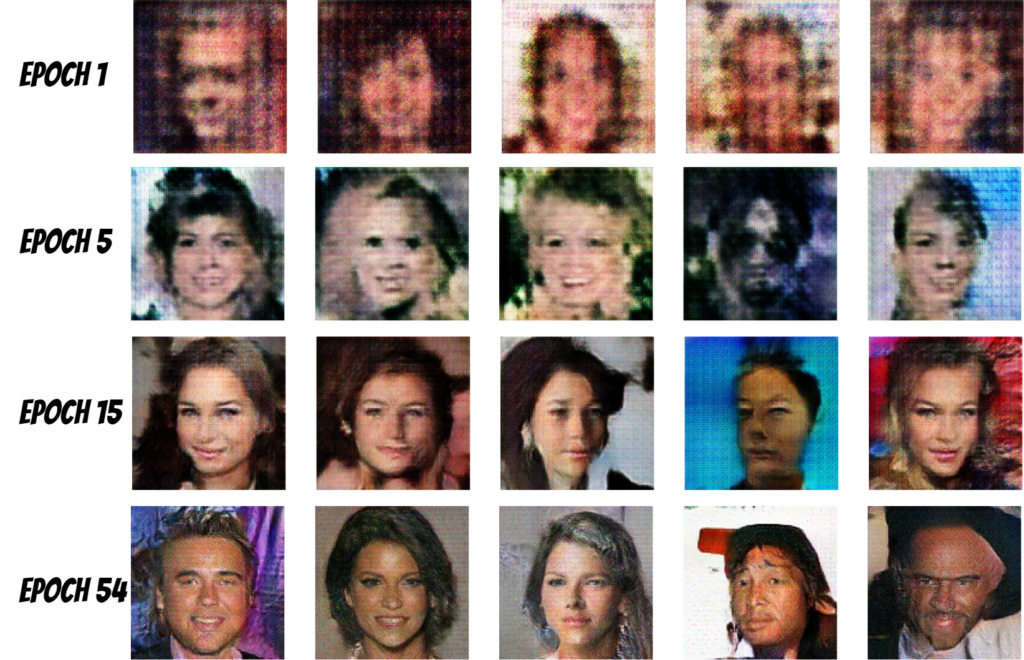
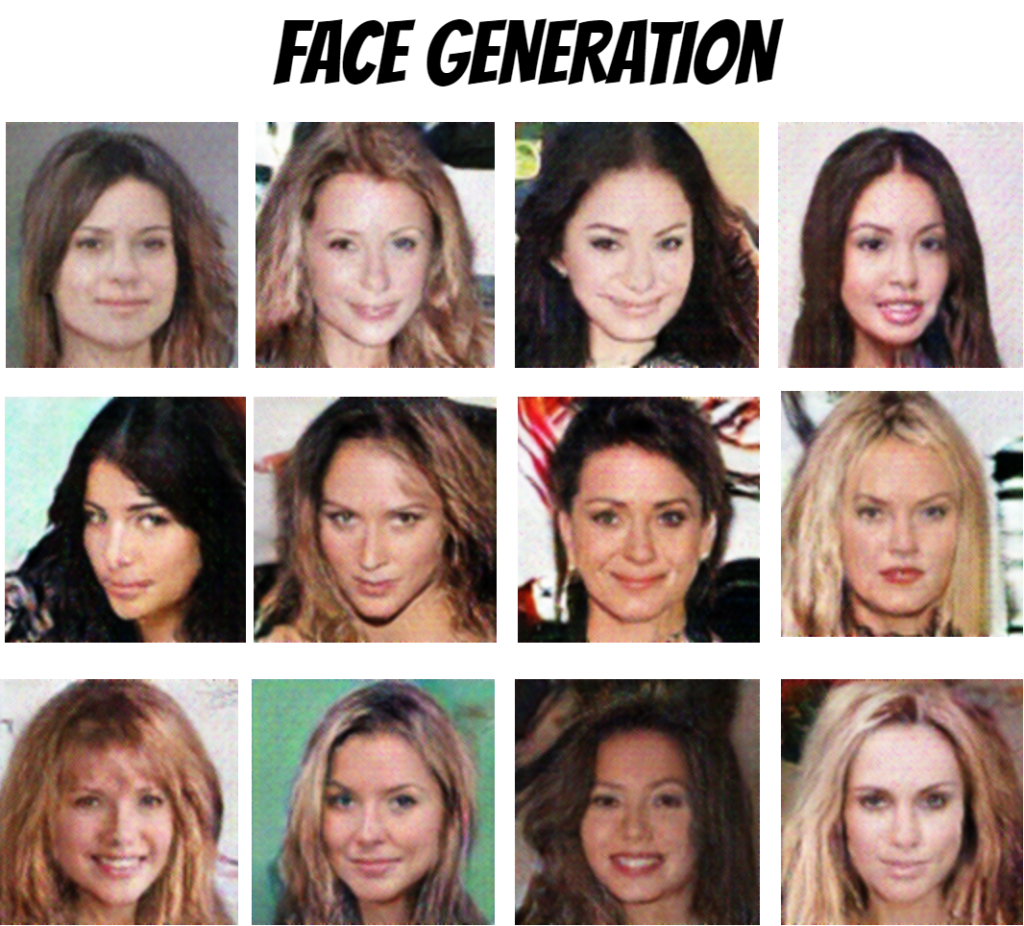
Finally, we can achieve the following results using DCGAN network.
As you can see some faces look realistic while some are distorted, additionally the network can only generate low resolution images.
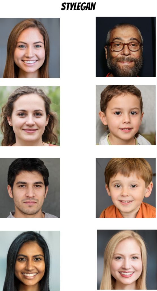
We can achieve much better results using the StyleGaN (arxiv article) network, which, among other things, differs in that the next layers of the network are progressively added during training.
I generated the images using pretrained networks and the effect is really amazing.
We use cookies to ensure that we give you the best experience on our website. If you continue to use this site we will assume that you are happy with it.Ok