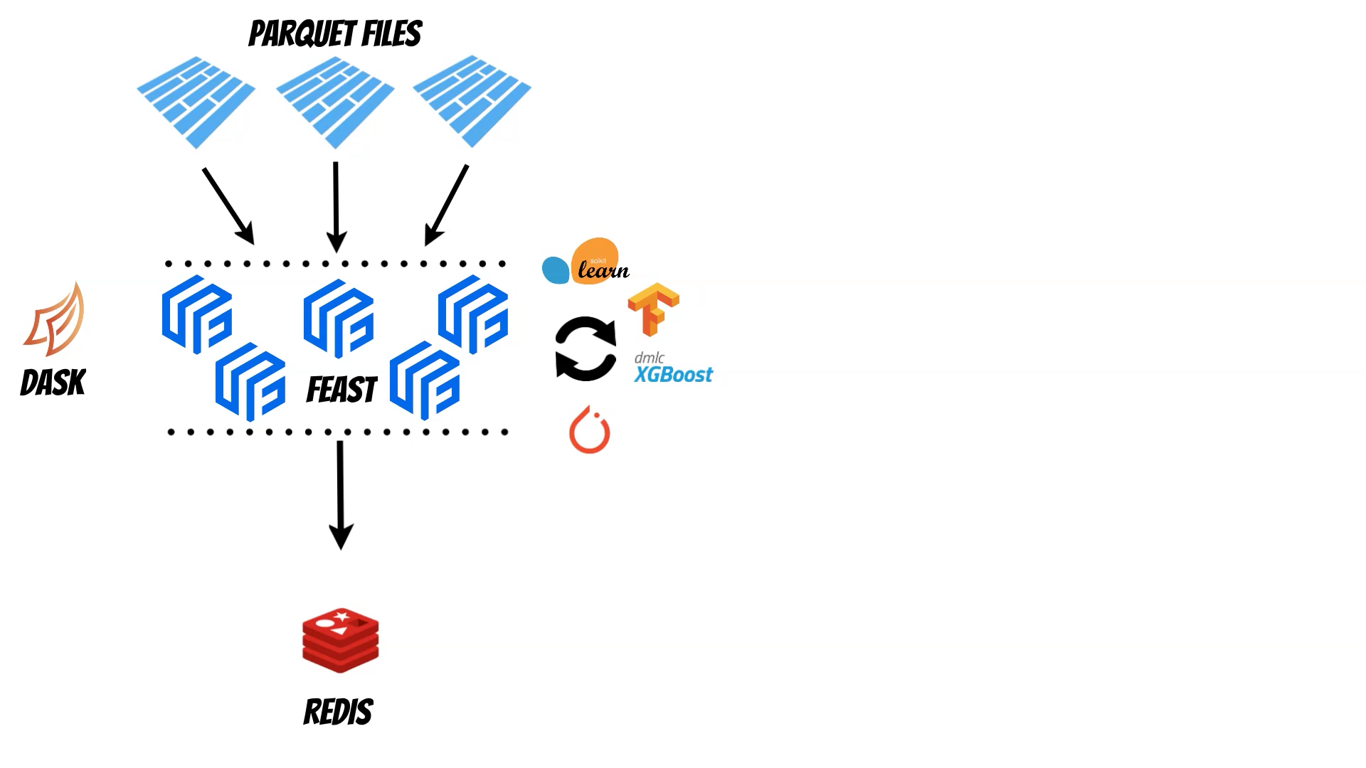
In this article I will show how we combine Feast and Dask library to create distributed feature store.
Before you will continue reading please watch short introduction:
The Feature Store is very important component of the MLops process which helps to manage historical and online features. With the Feast we can for example read historical features from the parquet files and then materialize them to the Redis as a online store.
But what to do if historical data size exceeds our machine capabilities ? The Dask library can help to solve this problem. Using Dask we can distribute the data and calculations across multiple machines. The Dask can be run on the single machine or on the cluster (k8s, yarn, cloud, HPC, SSH, manual setup). We can start with the single machine and then smoothly pass to the cluster if needed. Moreover thanks to the Dask we can read bunch of parquets using path pattern and evaluate distributed training using libraries like scikit-learn or XGBoost
I have prepared ready to use docker image thus you can simply reproduce all steps.
But with the docker you will have the whole environment ready.
In the notebook you will can find all the steps:
Random data generation
I have used numpy and scikit-learn to generate 1M entities end historical data (10 features generated with make_hastie_10_2 function) for 14 days which I save as a parquet file (1.34GB).
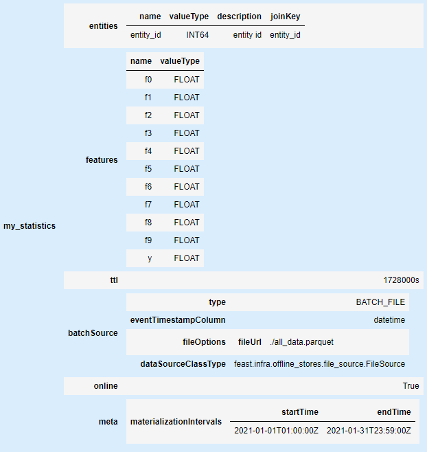
Feast configuration and registry
feature_store.yaml - where I use local registry and Sqlite database as a online store.
features.py - with one file source (generate parquet) and features definition.
The create the Feast registry we have to run:
feast apply
Additionally I have created simple library which helps to inspect feast schema directly in the Jupyter notebook
pip install feast-schema
from feast_schema import FeastSchema

FeastSchema('.').show_schema()
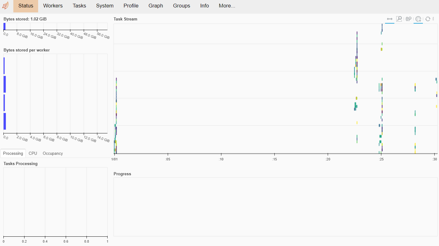
Dask cluster setup
Then I setup simple Dask cluster with scheduler and 4 workers.
Using Dask dataframe we can continue distributed training with the distributed data.
On the other hand if we will use Pandas dataframe the data will be computed to the one node.
To start distributed training with scikit-learn we can use Joblib library with the dask backend:
In this article I will show how to measure comments toxicity using Machine Learning models.
Before you will continue reading please watch short introduction:
Hate, rude and toxic comments are common problem in the internet which affects many people.
Today, we will prepare neural network,
which detects comments toxicity,
directly in the browser.
The goal is to create solution which will detect toxicity in the realtime and warn the user during writing,
which can discourage from writing toxic comments.
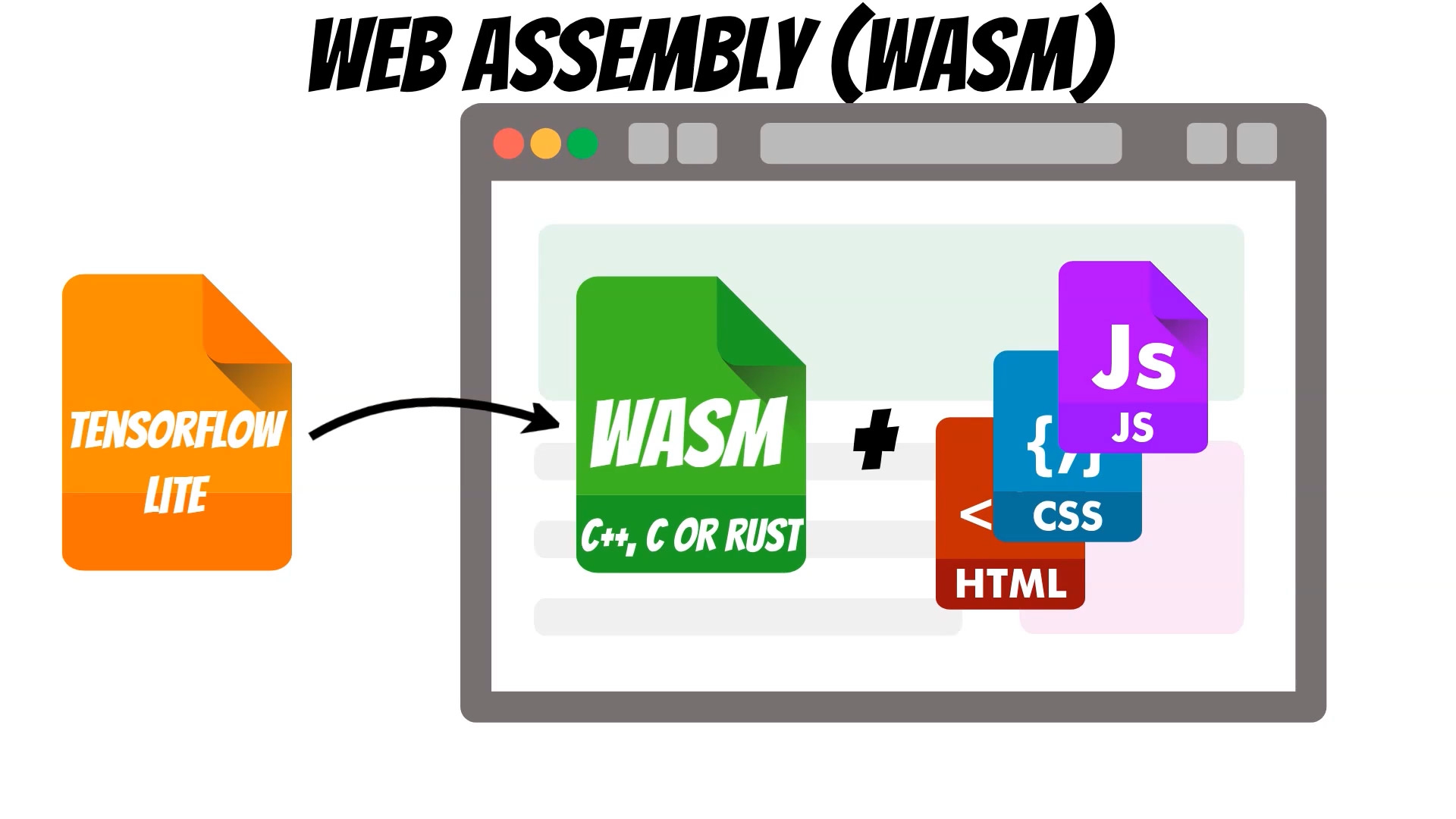
To do this, we will train the tensorflow lite model,
which will run in the browser using WebAssembly backend.
The WebAssembly (WASM) allows running C, C++ or RUST code at native speed.
Thanks to this, prediction performance will be better than running it using javascript tensorflowjs version.
Moreover, we can serve the model, on the static page, with no additional backend servers required.
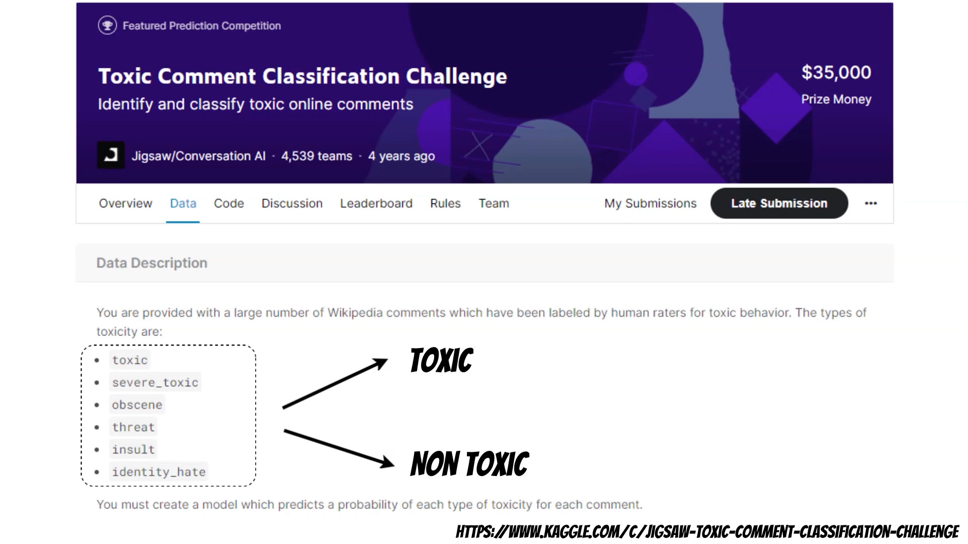
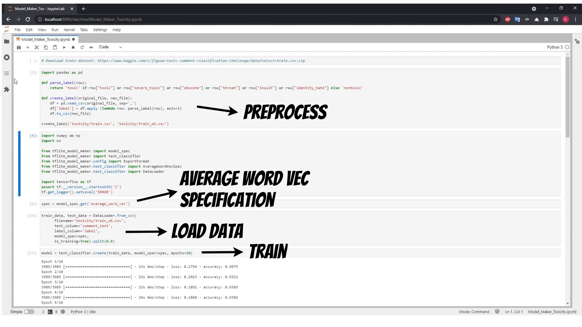
Our model, will only classify, if the text is toxic, or not. Thus we need to start with preprocessing training data. Then we will use the tensorflow lite model maker library.
We will also use the Averaging Word Embedding specification which will create words embeddings and dictionary mappings using training data thus we can train the model in the different languages.
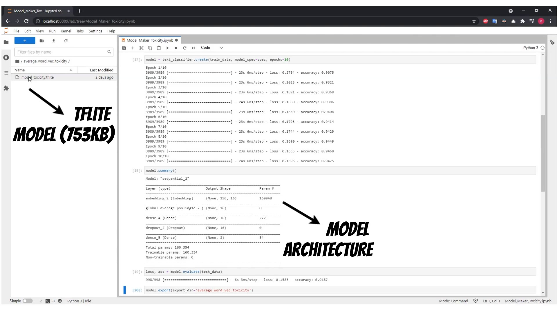
The Averaging Word Embedding specification based model will be small <1MB.
If we have small dataset we can use the pretrained embeddings. We can choose MobileBERT or BERT-Base specification.
In this case models will much more bigger 25MB w/ quantization 100MB w/o quantization for
MobileBERT and 300MB for BERT-Base (based on tutorial )
Using simple model architecture (Averaging Word Embedding), we can achieve about nighty five percent accuracy, and small model size, appropriate
for the web browser, and web assembly.
Now, let’s prepare the non-toxic forum web application,
where we can write the comments.
When we write non-toxic comments, the model won’t block it.
On the other hand, the toxic comments will be blocked,
and the user warned.
Of course, this is only client side validation, which can discourage users,
from writing toxic comments.
To run the example simply clone git repository and run simple server to serve the static page:
git clone https://github.com/qooba/ai-toxicless-texts.git
cd ai-toxicless-texts
python3 -m http.server
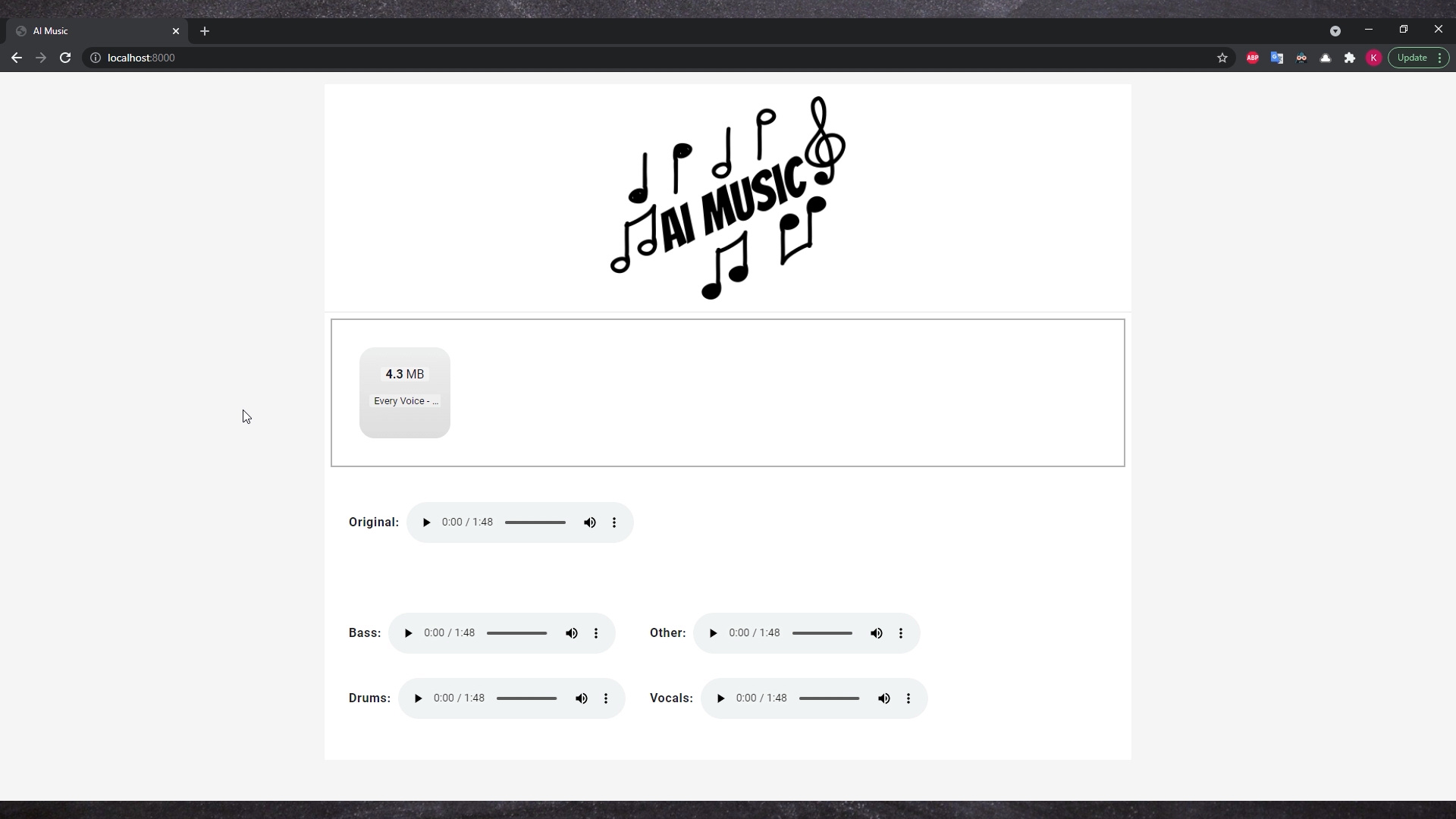
In this article I will show how we can extract music sources: bass, drums, vocals and other accompaniments using neural networks.
Before you will continue reading please watch short introduction:
Separation of individual instruments from arranged music is another area where machine learning
algorithms could help. Demucs solves this problem using neural networks.
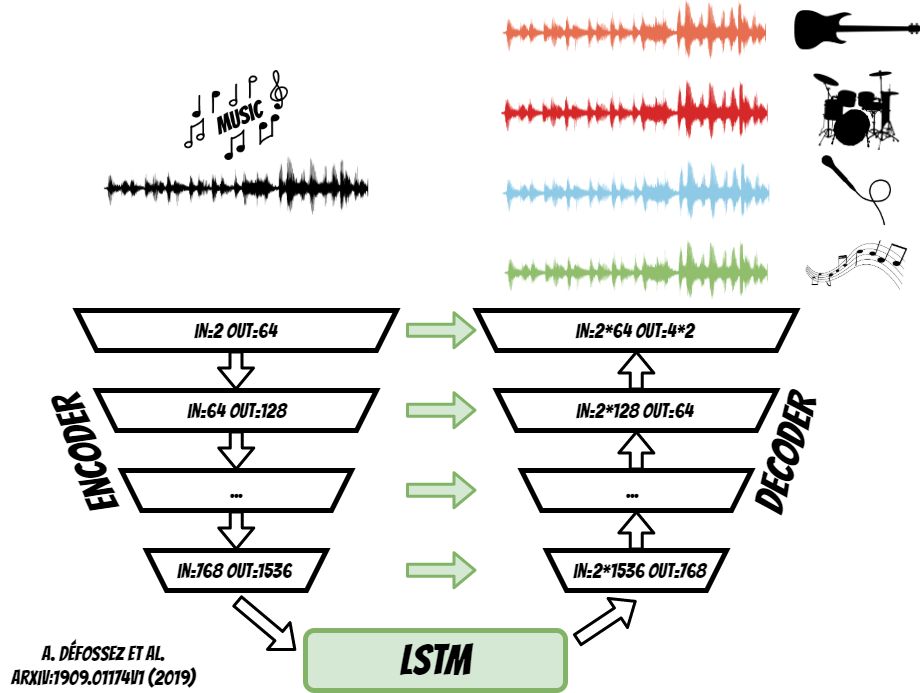
The trained model (https://arxiv.org/pdf/1909.01174v1.pdf) use U-NET architecture which contains two parts encoder and decoder.
On the encoder input we put the original track and after processing we get bass, drums, vocals and other accompaniments at the decoder output.
The encoder, is connected to the decoder,
through additional LSTM layer,
as well as residual connections between subsequent layers.
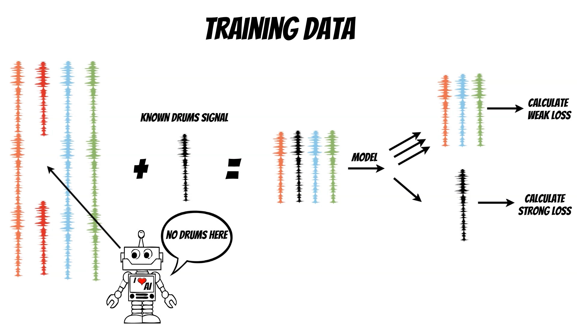
Ok, we have neural network architecture but what about the training data ?
This is another difficulty which can be handled by the unlabeled data remixing pipeline.
We start with another classifier, which can find the parts of music,
which do not contain the specific instruments, for example drums.
Then, we mix it with well known drums signal, and separate the tracks
using the model.
Now we can compare, the separation results, with known drums track and mixture of other instruments.
According to this, we can calculate the loss (L1 loss), and use it during the training.
Additionally, we set different loss weights, for known track and the other.
The whole UI is kept in the docker image thus you can simply try it:
#for CPU
docker run --name aiaudioseparation -it -p 8000:8000 -v $(pwd)/checkpoints:/root/.cache/torch/hub/checkpoints --rm qooba/aimusicseparation

#for GPU
docker run --name aiaudioseparation --gpus all -it -p 8000:8000 -v $(pwd)/checkpoints:/root/.cache/torch/hub/checkpoints --rm qooba/aimusicseparation
In this article I will show how we can prepare and perform calculations on quantum computers
using OpenFermion, Cirq and PySCF.
Before you will continue reading please watch short introduction:
Currently, there are many supercomputing centers, where we can run complicated simulations.
However, there are still problems that are beyond the capabilities of classical computers,
which can be addressed by quantum computers.
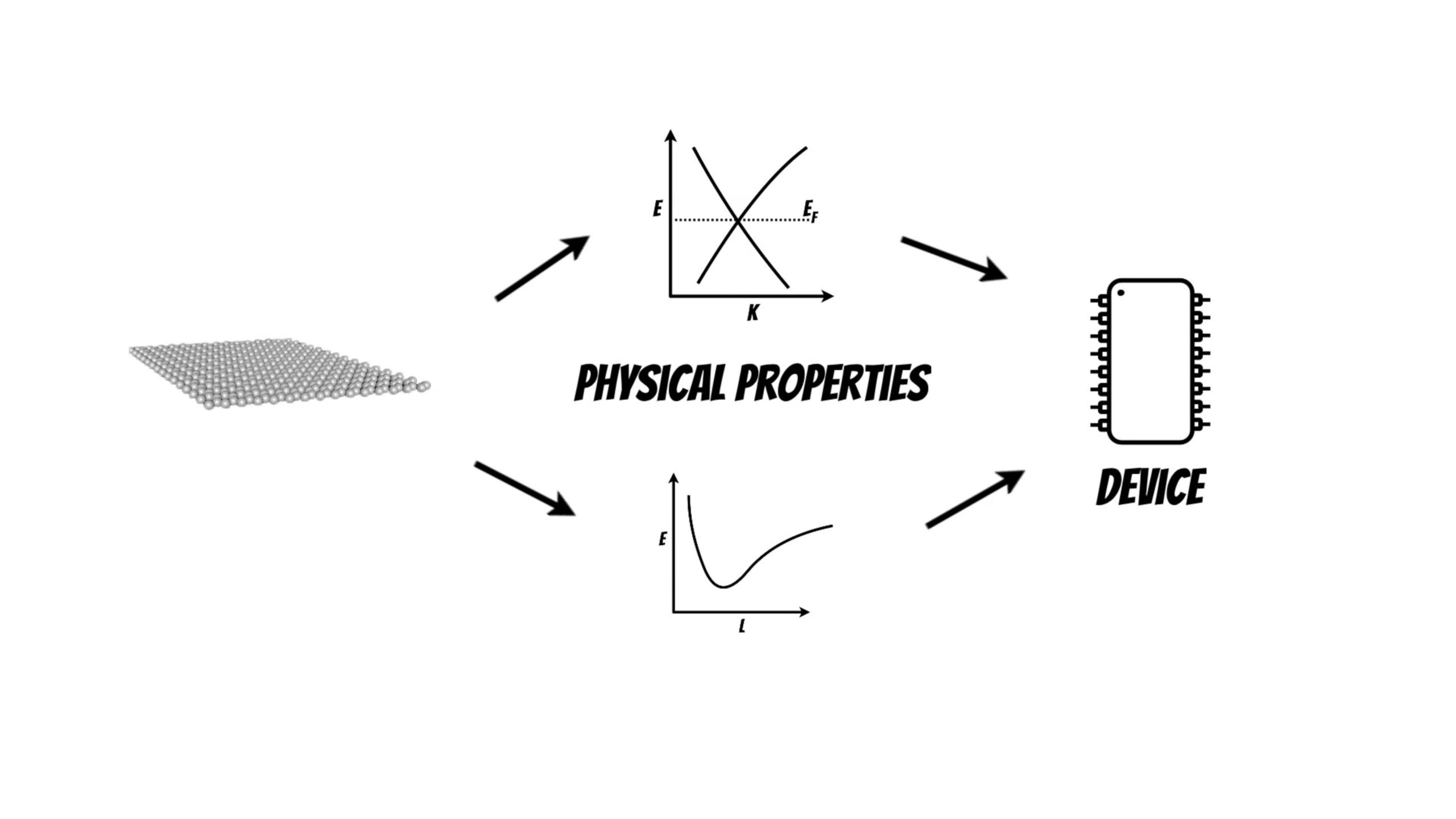
Quantum chemistry and materials science problems which that are described by the laws of
quantum mechanics can be mapped to the quantum computers and projected to qubits.
OpenFermion is the library which can help to perform such calculations on a quantum computer.
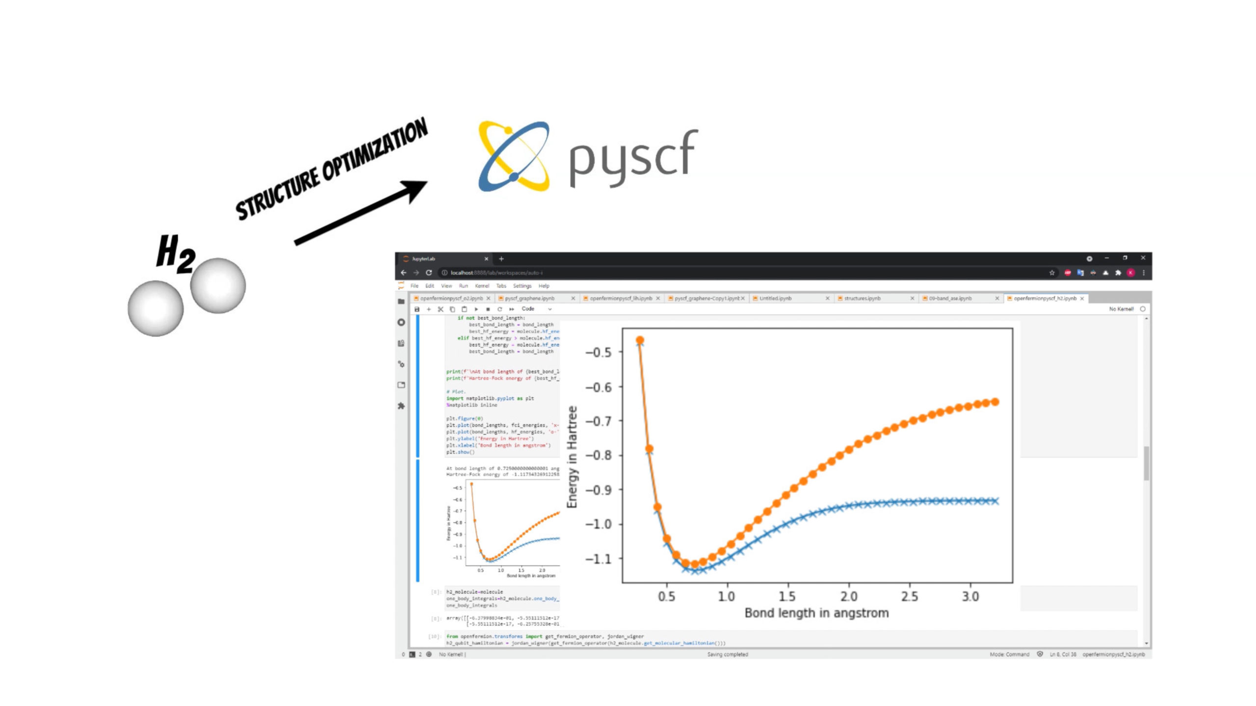
Additionally we will use the PySCF package which will help to perform initial structure optimization (if you are interested in PySCF package I have shared the example DFT based band structure calculation of the single layer graphene structure pyscf_graphene.ipynb).
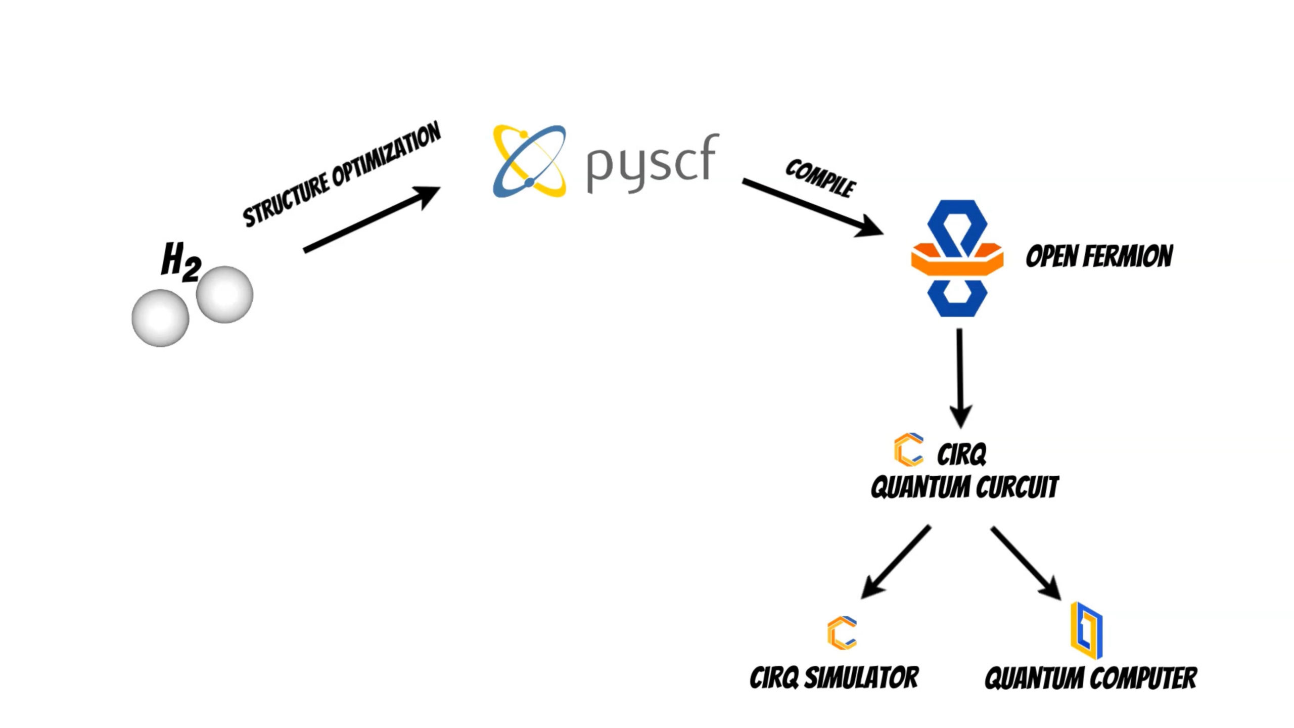
In our example we will investigate [latex]H_2[/latex] molecule for simplicity. We will use the PySCF package to find optimal bond length of the molecule.
Thanks to the OpenFermion-PySCF plugin we can smoothly use the molecule initial state obtained from PySCF package run in OpenFermion library (openfermionpyscf_h2.ipynb).
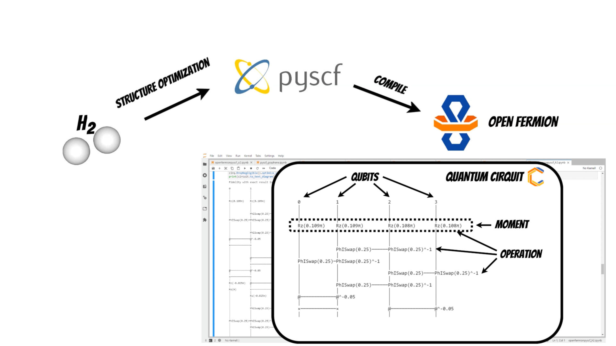
Now it is time to compile the molecule to the representation readable by the quantum computer
using OpenFermion and Cirq library.
Currently you can use several methods to achieve this:
Using one of this methods we get optimized quantum circuit.
In our case the quantum cirquit for [latex]H_2[/latex] system will be represented by 4 qubits and operations that act on them (moment is collection of operations that act at the same abstract time slice).
Before you will continue reading please watch short introduction:
In the last article (TinyML with Arduino) I have shown the example TinyML model which will classify
jelly bears using RGB sensor.
The next step, will be to build a process that will simplify, the model versions management, and the deployment.
–device=/dev/ttyACM0 - is arduino device connected using USB
AWS_ACCESS_KEY_ID and AWS_SECRET_ACCESS_KEY - are minio credentials
MLFLOW_S3_ENDPOINT_URL - is minio url
MLFLOW_TRACKING_URI - is mlflow url
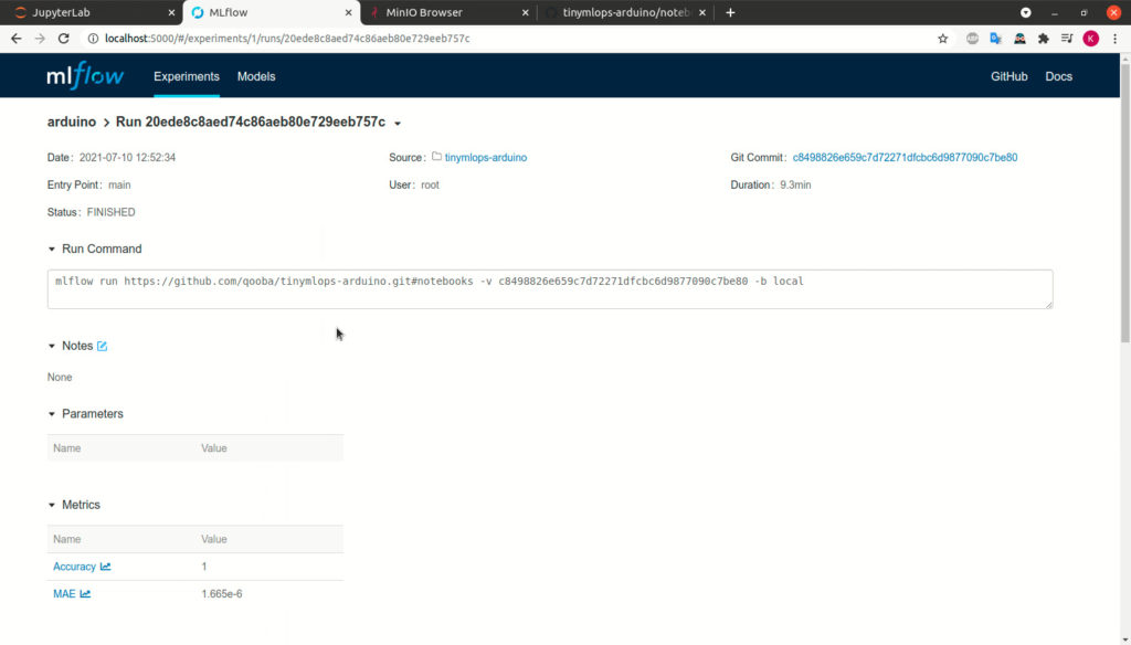
${RUN_ID} - is run id of model saved in MLflow registry
Additionally we have several command line options:
ARDUINO MLOPS

Syntax: docker run -it qooba/tinyml-arduino:mlops -h [-r MLFLOW_RUN_ID] [-s ARDUINO_SERIAL] [-c ARDUINO_CORE] [-m ARDUINO_MODEL]
options:
-h|--help     Print help
-r|--run      MLflow run id
-s|--serial   Arduino device serial (default: /dev/ttyACM0)
-c|--core     Arduino core (default: arduino:mbed_nano)
-m|--model    Arduino model (default: arduino:mbed_nano:nano33ble)
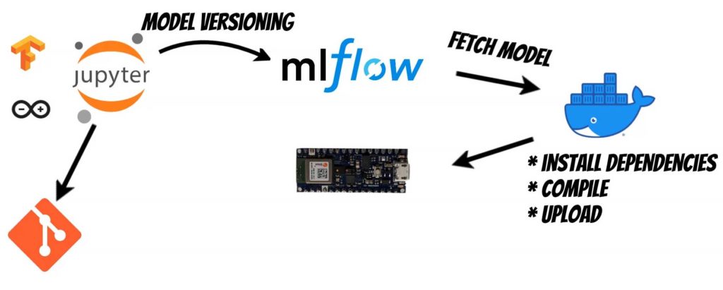
After running the code the docker image qooba/tinyml-arduino:mlops
will fetch the model for indicated RUN_ID from MLFlow.
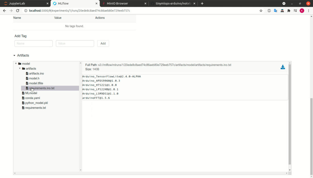
Then it will install required dependencies using the file requirements.ino.txt.
It will compile the model and the Arduino code.
And finally upload it to the device.
Thanks to this, we can more easily manage subsequent versions of models, and automate the deployment process.
We use cookies to ensure that we give you the best experience on our website. If you continue to use this site we will assume that you are happy with it.Ok