In this video I will show how to generate and
use graph embeddings with feature store.
Before you will continue reading please watch short introduction:
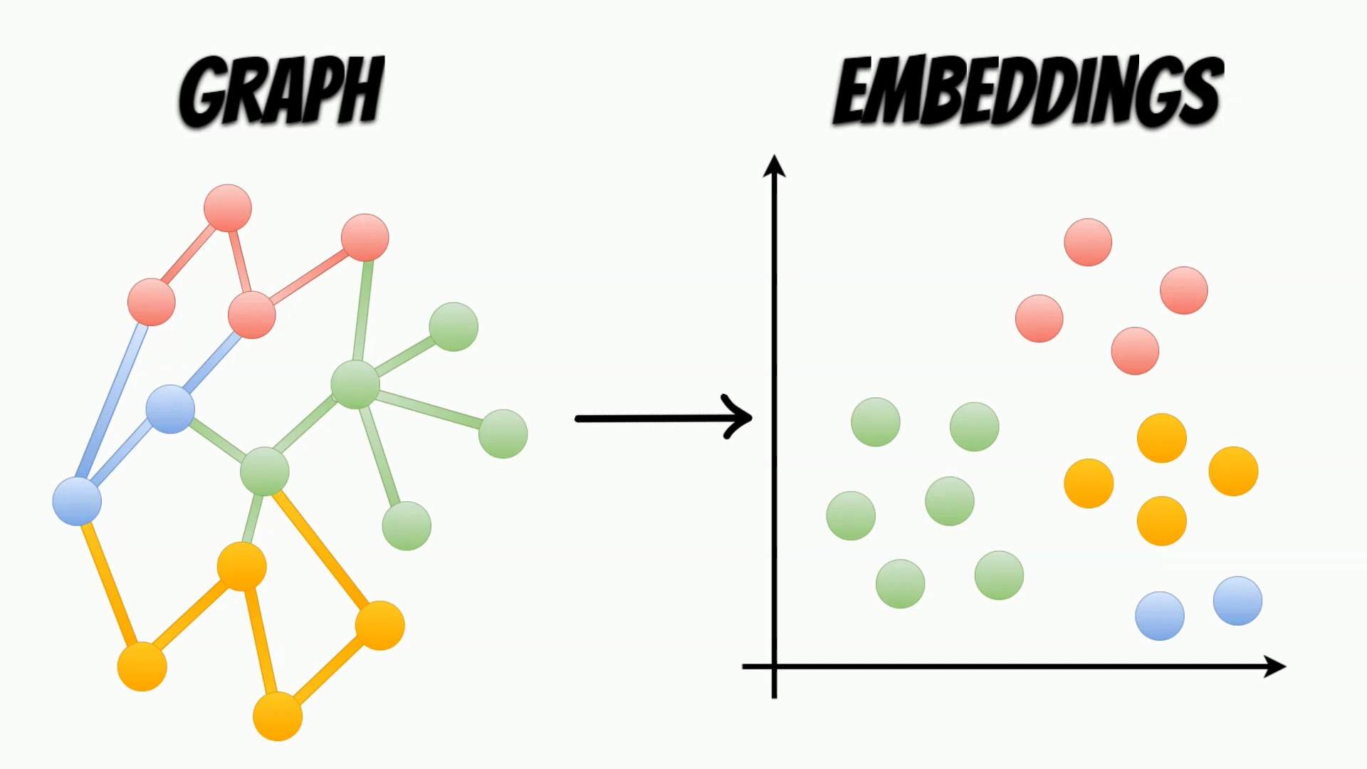
Graphs are structures, which contain sets of entity nodes and edges,
which represent the interaction between them.
Such data structures, can be used in many areas like social networks,
web data, or even molecular biology, for modeling real-life interactions.
To use properties contained in the graphs, in the machine learning algorithms,
we need to map them, to more accessible representations, called embeddings.
In contrast to the graphs, the embeddings are structures, representing the nodes features,
and can be easily used, as an input of the machine learning algorithms.
Because graphs are frequently represented by the large datasets,
embeddings calculation can be challenging. To solve this problem,
I will use a very efficient open source project,
Cleora which is entirely written in rust.
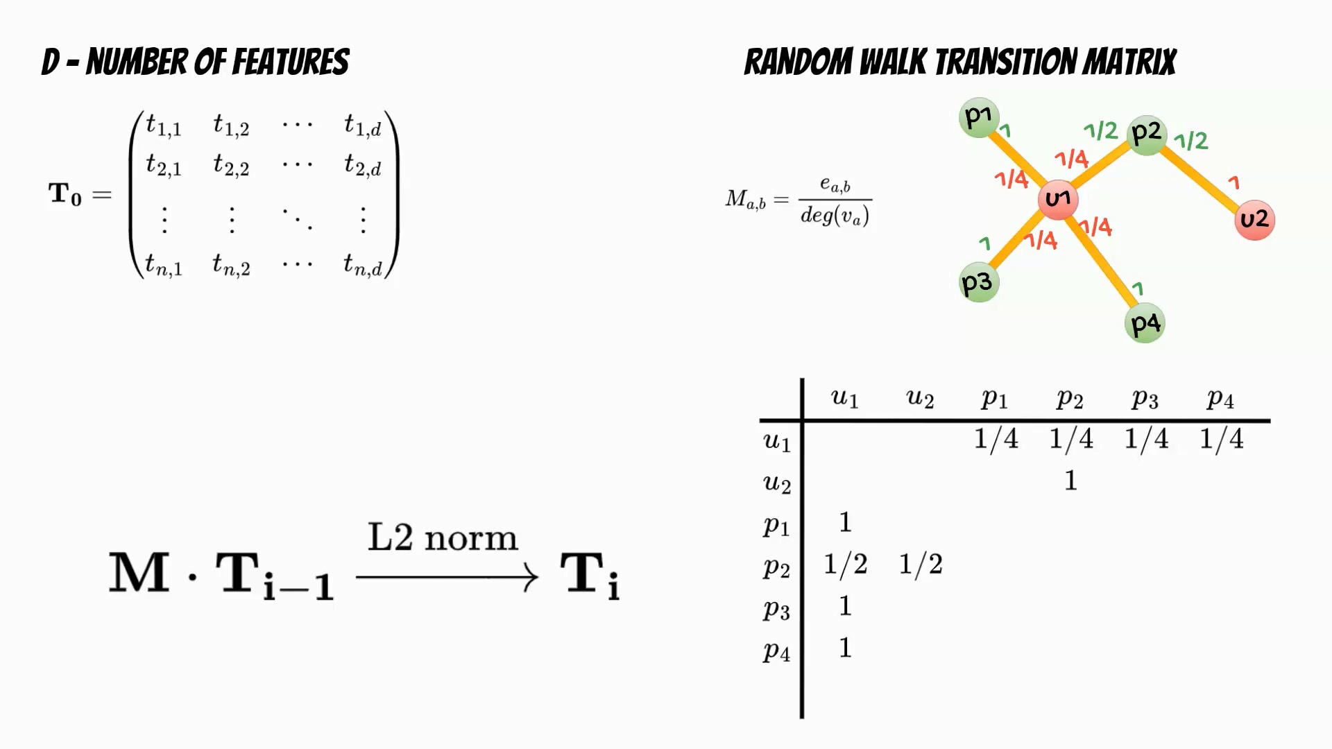
Let’s follow the Cleora algorithm. In the first step we need to determine
the number of features which will determine the embedding dimensionality.
Then we initialize the embeddings matrix. In the next step based on
the input data we calculate the random walk transition matrix.
The matrix describes the relations between nodes and is defined
as a ratio of number of edges running from first to second node,
and the degree of the first node.
The training phase is iterative multiplication of the embeddings matrix
and the transition matrix followed by L2 normalization of the embeddings rows.
Finally we get embedding matrix for the defined number of iterations.
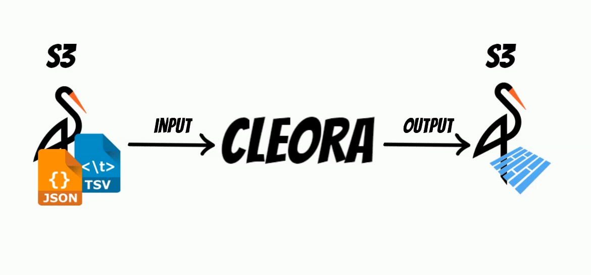
Moreover, to be able to simply build a solution, I have extended the project,
with possibility of reading and writing to S3 store, and Apache Parquet format usage,
which significantly reduce embedding size.
Additionally, I have wrapped the rust code, with the python bindings,
thus we can simply install it and use it as a python package.
Based on the Cleora example,
I will use the Facebook dataset from
SNAP,
to calculate embeddings from page to page graph, and train a machine learning model,
which classifies page category.
For each node, I have added an additional column datetime which represents timestamp,
and will help to check how calculated embeddings, will change over time.
Additionaly every embeddings recalculation will be saved as
a separate parquet file eg. emb__CliqueNode__CliqueNode_20220910T204145.parquet.
Thus we will be able to follow embeddings history.
Now, we are ready to consume the calculated embeddings,
with Feast feature store, and Yummy extension.
from datetime import timedelta
from feast import Entity, Field, FeatureView
from yummy import ParquetSource
from feast.types import Float32, Int32

my_stats_parquet = ParquetSource(
    name="my_stats",
    path="s3://output/emb__CliqueNode__CliqueNode_*.parquet",
    timestamp_field="datetime",
    s3_endpoint_override="http://minio:9000",
)

my_entity = Entity(name="entity", description="entity",)

schema = [Field(name="entity", dtype=Int32)] + [Field(name=f"f{i}", dtype=Float32) for i in range(0,1024)]

mystats_view_parquet = FeatureView(
    name="my_statistics_parquet",
    entities=[my_entity],
    ttl=timedelta(seconds=3600*24*20),
    schema=schema,
    online=True, source=my_stats_parquet, tags={},)
Then we apply feature store definition:
feast apply
Now we are ready to fetch ebeddings for defined timestamp.
from feast import FeatureStore
import polars as pl
import pandas as pd
import time
import os
from datetime import datetime
import yummy

store = FeatureStore(repo_path=".")
start_time = time.time()

features = [f"my_statistics_parquet:f{i}" for i in range(0,1024)]

training_df = store.get_historical_features(
    entity_df=yummy.select_all(datetime(2022, 9, 14, 23, 59, 42)),
    features = features,
).to_df()

print("--- %s seconds ---" % (time.time() - start_time))
training_df
Then we prepare training data for data for the SNAP dataset:
import numpy as np
from sklearn.model_selection import train_test_split
df = pd.read_csv("../facebook_large/musae_facebook_target.csv")

classes = df['page_type'].unique()
class_ids = list(range(0, len(classes)))
class_dict = {k:v for k,v in zip(classes, class_ids)}
df['page_type'] = [class_dict[item] for item in df['page_type']]

train_filename = "fb_classification_train.txt"
test_filename = "fb_classification_test.txt"

train, test = train_test_split(df, test_size=0.2)

training_df=training_df.astype({"entity": "int32"})

entities = training_df["entity"].to_numpy()

train = train[["id","page_type"]].to_numpy()
test = test[["id","page_type"]].to_numpy()

df_embeddings=training_df.drop(columns=["event_timestamp"])\
    .rename(columns={ f"f{i}":i+2 for i in range(1024) })\
    .rename(columns={"entity": 0}).set_index(0)

valid_idx = df_embeddings.index.to_numpy()
train = np.array(train[np.isin(train[:,0], valid_idx) & np.isin(train[:,1], valid_idx)])
test = np.array([t for t in test if (t[0] in valid_idx) and (t[1] in valid_idx)])
Finally, we will train page classifiers.
from sklearn.linear_model import SGDClassifier
from sklearn.metrics import f1_score
from tqdm import tqdm
epochs=[20]
batch_size = 256
test_batch_size = 1000
embeddings=df_embeddings
y_train = train[:, 1]
y_test = test[:, 1]

clf = SGDClassifier(random_state=0, loss='log_loss', alpha=0.0001)
for e in tqdm(range(0, max(epochs))):
    for idx in range(0,train.shape[0],batch_size):
        ex=train[idx:min(idx+batch_size,train.shape[0]),:]
        ex_emb_in = embeddings.loc[ex[:,0]].to_numpy()
        ex_y = y_train[idx:min(idx+batch_size,train.shape[0])]
        clf.partial_fit(ex_emb_in, ex_y, classes=[0,1,2,3])

    if e+1 in epochs:
        acc = 0.0
        y_pred = []
        for n, idx in enumerate(range(0,test.shape[0],test_batch_size)):
            ex=test[idx:min(idx+test_batch_size,train.shape[0]),:]
            ex_emb_in = embeddings.loc[ex[:,0]].to_numpy()
            pred = clf.predict_proba(ex_emb_in)
            classes = np.argmax(pred, axis=1)
            y_pred.extend(classes)

        f1_micro = f1_score(y_test, y_pred, average='micro')
        f1_macro = f1_score(y_test, y_pred, average='macro')
        print(' epochs: {}, micro f1: {}, macro f1:{}'.format( e+1, f1_micro, f1_macro))
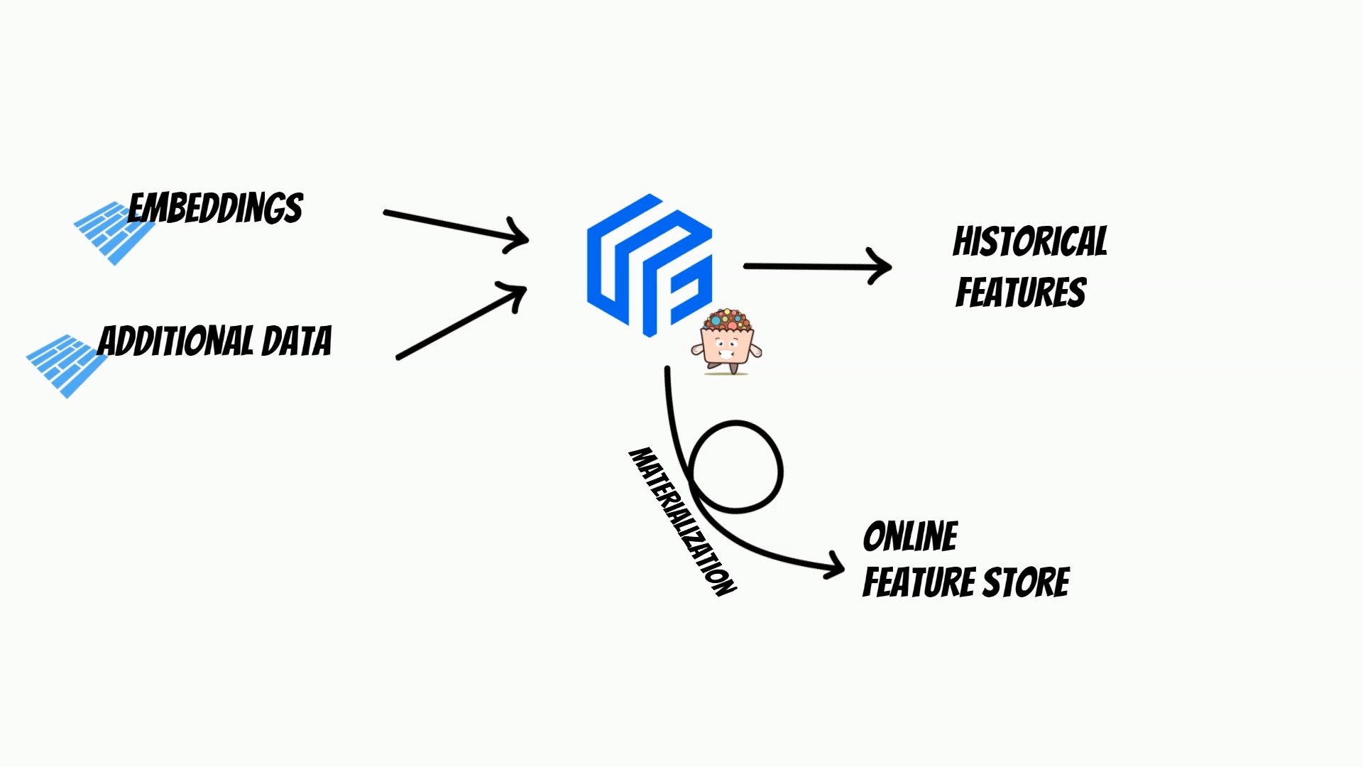
Because feature store can merge multiple sources,
we can easily enrich graph embeddings, with additional
features like additional page information.
We can also track, embeddings historical changes.
Moreover, using feature store we can materialize embeddings
to online store, which simplifies building a comprehensive MLOps process.
You can find the whole example.ipynb
on github and yummy documentation.
In this video I will show how to use Apache Iceberg as a store for historical feature store.
Moreover we will build end to end real-time ingestion example with:
Postgres
Kafka connect
Iceberg on Minio
Feast with Yummy extension
Before you will continue reading please watch short introduction:
Apache Iceberg, is an high-performance table format, which can be used for huge analytic datasets.
Iceberg offers several features like: schema evolution, partition evolution and hidden partitioning,
and many more, which can be used to effectively process, petabytes of data.
Read more
if you want to learn more about Iceberg features and how it compares to the other lake formats (Delta Lake and Hudi).
Apache Iceberg, is perfect candidate to use as an historical store thus
I have decided to integrate it, with the Feast feature store through,
Yummy extension.
To show how to use it I will describe end to end solution with
the real-time Iceberg ingestion from the other data sources.
To do this, I will use Kafka connect, with Apache Iceberg Sink
This can be used, to build Iceberg lake on on-premise s3 store,
or to move your data and build a feature store in the cloud.
You can follow the solution in the notebook: example.ipynb
and simply reproduce using docker.
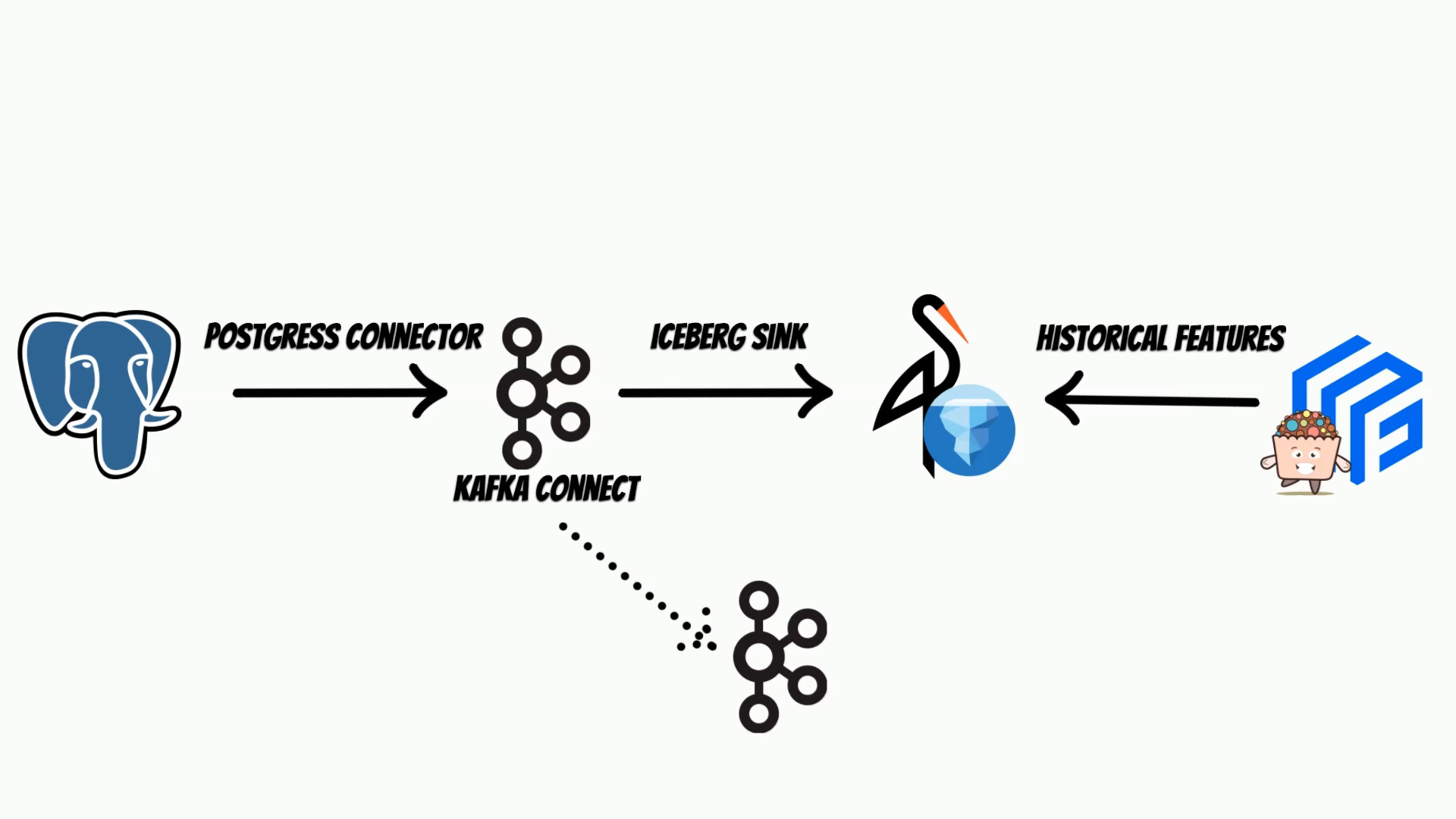
Suppose, we have our transactional system based on the postgres database,
where we keep current clients features.
We will track features changes, to build historical feature store.
The Kafka Connect, will use debezium postgres connector,
to track every data change and put it to the Iceberg using Iceberg sink.
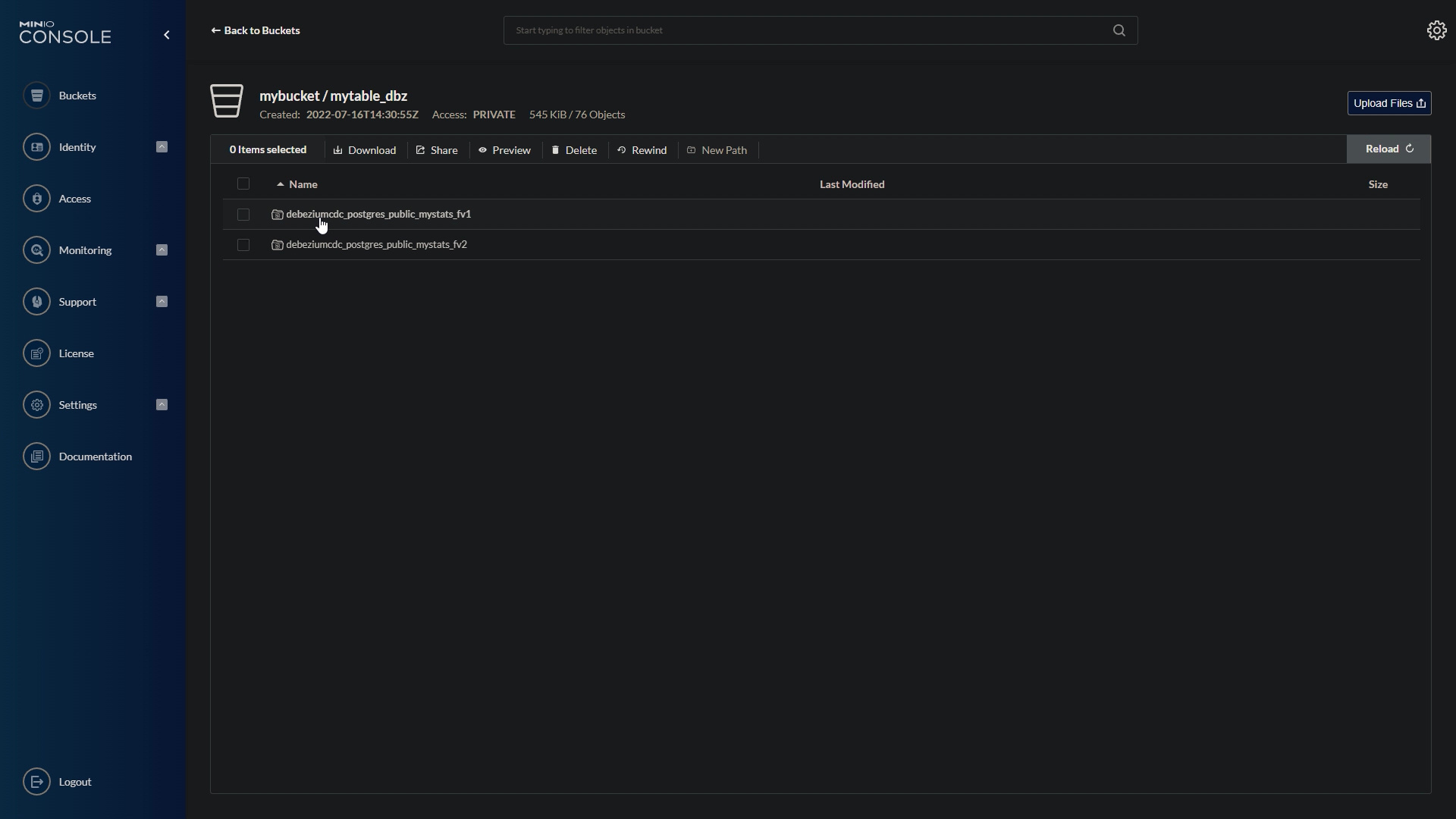
We will store iceberg tables, on the minio s3 store,
but of course you can use AWS S3.
Kafka Connect, is based on Kafka, thus we will also need a Kafka instance and zookeeper.
We will setup selected components using docker.
To start clone the repository:
git clone https://github.com/yummyml/yummy-iceberg-kafka-connect.git
cd yummy-iceberg-kafka-connect
All below commands are already in the example.ipynb
notebook but I will explain all of them.
Kafka Connect, will publish database changes to the kafka, thus we also need to create appropriate topics,
if we don’t have topics auto-creation enabled.
I have created two topics because we will track the two postgress tables.
Now, we can setup a postgres connector, and Iceberg sink through, Kafka connect api.
In the postgres connector, we need to specify a list of tables, which we want to track.
Currently, you can use Iceberg, only with the spark backend.
You can also, add additional spark configuration, such as catalog configuration or
s3 store configuration.
In the next step, you have to add Iceberg Data Source.
In the feature store definition, you specify a path to the iceberg table or table name, which you want to consume on filesystem or s3 store respectively.
Of course, you can combine the Iceberg data source, with the other data sources like parquets, csv files or even delta lake if needed.
Here you see how to do this.
Now, we are ready to apply feature store definition, and fetch historical features.
In this article I’d like to show how to predict video matte using machine learning model.
Before you will continue reading please watch short introduction:
In the previous article I have shown how to cut the background from the image:
AI Scissors – sharp cut with neural networks.
This time we will generate matte for video without green box using machine learning model.
Video matting, is a technique which helps to separate video into two or more layers, for example foreground and background.
Using this method, we generate alpha matte, which determine the boundaries between the layers,
and allows for example to substitute the background.
Nowadays these methods, are widely used in video conference software, and probably you know it very well.
But is it possible, to process 4K video and generate a high resolution alpha matte, without green screen props ?
Following the article: arxiv 2108.11515 we can achieve this using:
“The Robust High-Resolution Video Matting with Temporal Guidance method”.
The authors, have used recurrent architecture to exploit temporal information. Thus the model predictions,
are more coherent and this improves matting robustness.
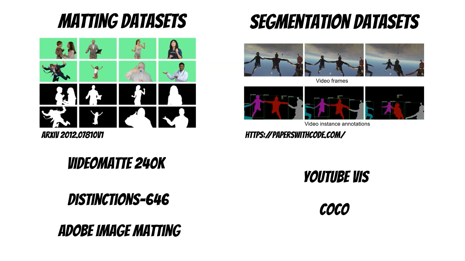
Moreover, their proposed new training strategy, where they use both matting (VideoMatte240K, Distinctions-646, Adobe Image Matting)
and segmentation datasets (YouTubeVIS, COCO).
This mixture helps to achieve better quality, for complex datasets and prevents overfitting.
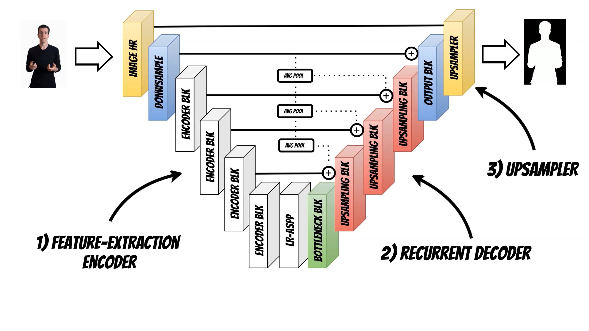
Neural network architecture, consists of three elements.
The first element is Feature-Extraction Encoder, which extracts individual frames features, especially accurately locating human subjects. The encoder, is based on the MobileNetV3-Large backbone.
The second element is Recurrent Decoder, that aggregates temporal information. Recurrent approach helps to learn, what information to keep and forget by itself, on a continuous stream of video.
And Finally Deep Guided Filter module for high-resolution upsampling.
Because the authors shared their work and models, I have prepared an easy to use docker based application which we can use to simply process your video.
To run it you will need docker and you can run it with GPU or without GPU card.
With GPU:
docker run -it --gpus all -p 8000:8000 --rm --name aimatting qooba/aimatting:robust
Without GPU:
docker run -it -p 8000:8000 --rm --name aimatting qooba/aimatting:robust
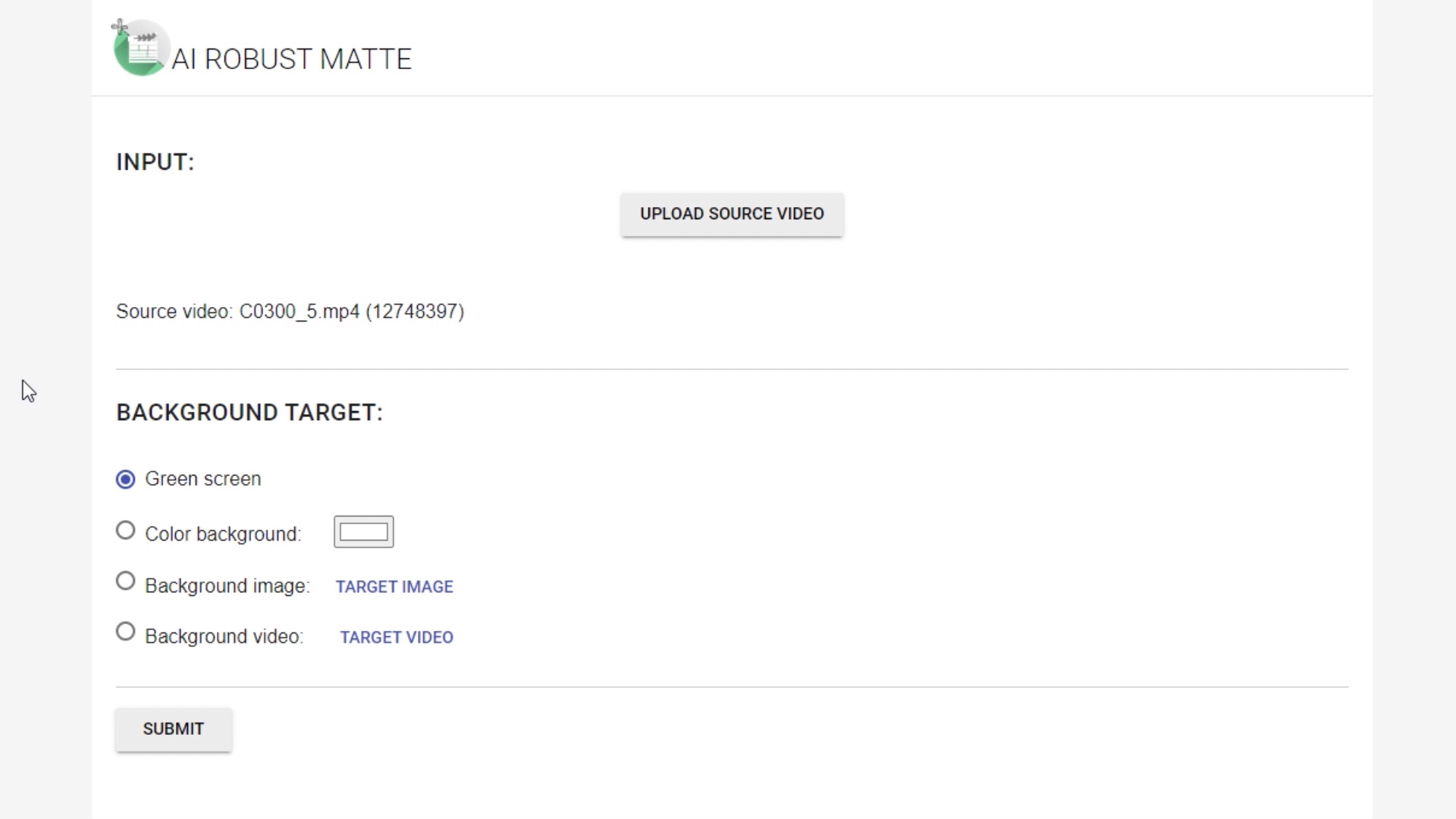
Then open address http://localhost:8000/ in your browser.
Because the model does not require any auxiliary inputs such as a trimap or a pre-captured background image we simply upload our video and choose required the background. Currently we can generate green screen background which can be then replaced in the video editing software.
We can also use predefined color, image or even video.
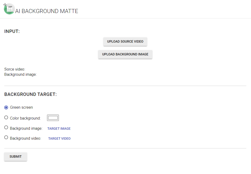
I have also prepared the app for the older algorithm version:
arxiv 2012.07810
To use please run:
docker run -it --gpus all -p 8000:8000 --rm --name aimatting qooba/aimatting:background
This version additionally requires the background image but sometimes achieves better results.
In this article I’d like to present a really delicious Feast extension Yummy.
Before you will continue reading please watch short introduction:
Last time I showed the Feast integration with the Dask
framework which helps to distribute ML solutions across the cluster
but doesn’t solve other problems.
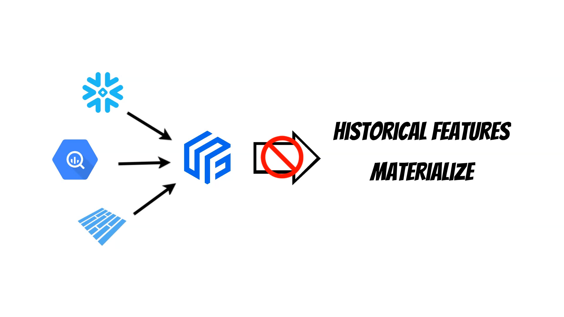
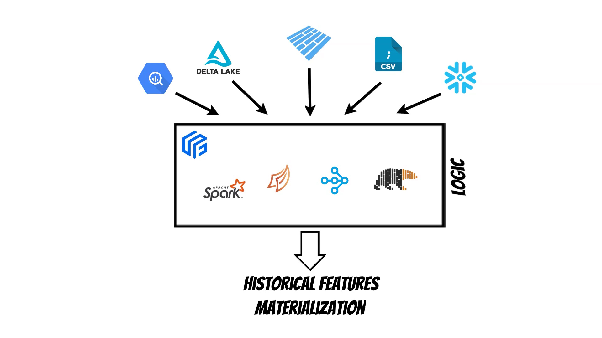
Currently in Feast we have a warehouse based approach where Feast builds
and executes query appropriate for specific database engines.
Because of this architecture Feast can’t use multiple data sources
at the same time.
Moreover the logic which fetch historical features from offline data sources
is duplicated for every datasource implementation which makes it difficult to
maintain.
To solve this problems I have decided to create
Yummy
Feast extension, which is also published
as a pypi package.
In Yummy I have used a backend based approach which centralizes the
logic which fetches historical data from offline stores.
Currently: Spark, Dask,
Ray and Polars
backends are supported.
Moreover because the selected backend is responsible for joining the data we can use
multiple different data sources at the same time.
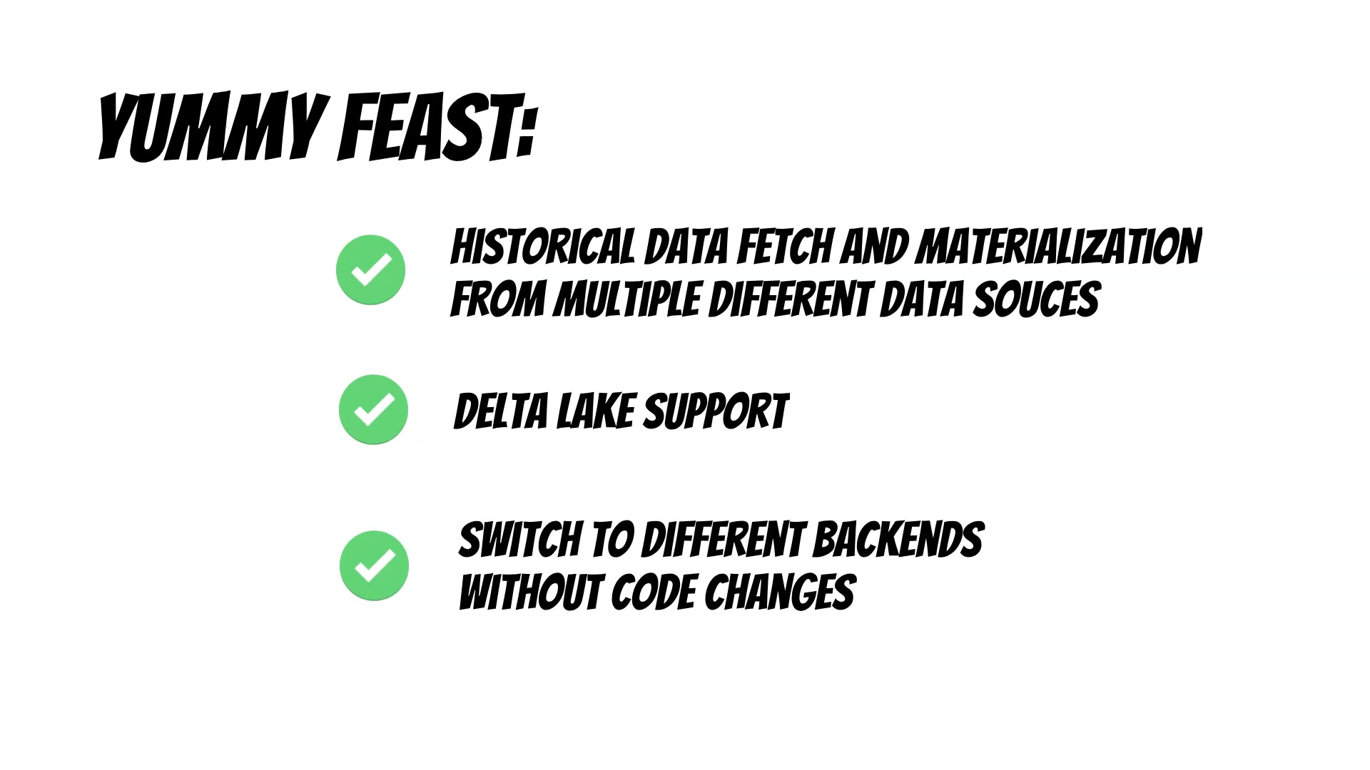
Additionally with Yummy we can start using a feature store on a single machine and then
distribute it using the selected cluster type.
We can also use ready to use platforms like: Databricks,
Coiled, Anyscale to scale our solution.
To use Yummy we have to install it:
pip install yummy
Then we have to prepare Feast configuration feature_store.yaml:
In this case we will use s3 as a feature store registry and redis as an online store.
The Yummy takes offline store responsibility and in this case we have selected
dask backend.
For dask, ray and polars backends we don’t have to set up the cluster to
work. In this case if we don’t provide cluster configuration they will run
locally. For Apache Spark additional configuration is required for local machines.
In the next step we need to provide feature store definition in the python file eg.
features.py
In this article I will show how we combine Feast and Dask library to create distributed feature store.
Before you will continue reading please watch short introduction:
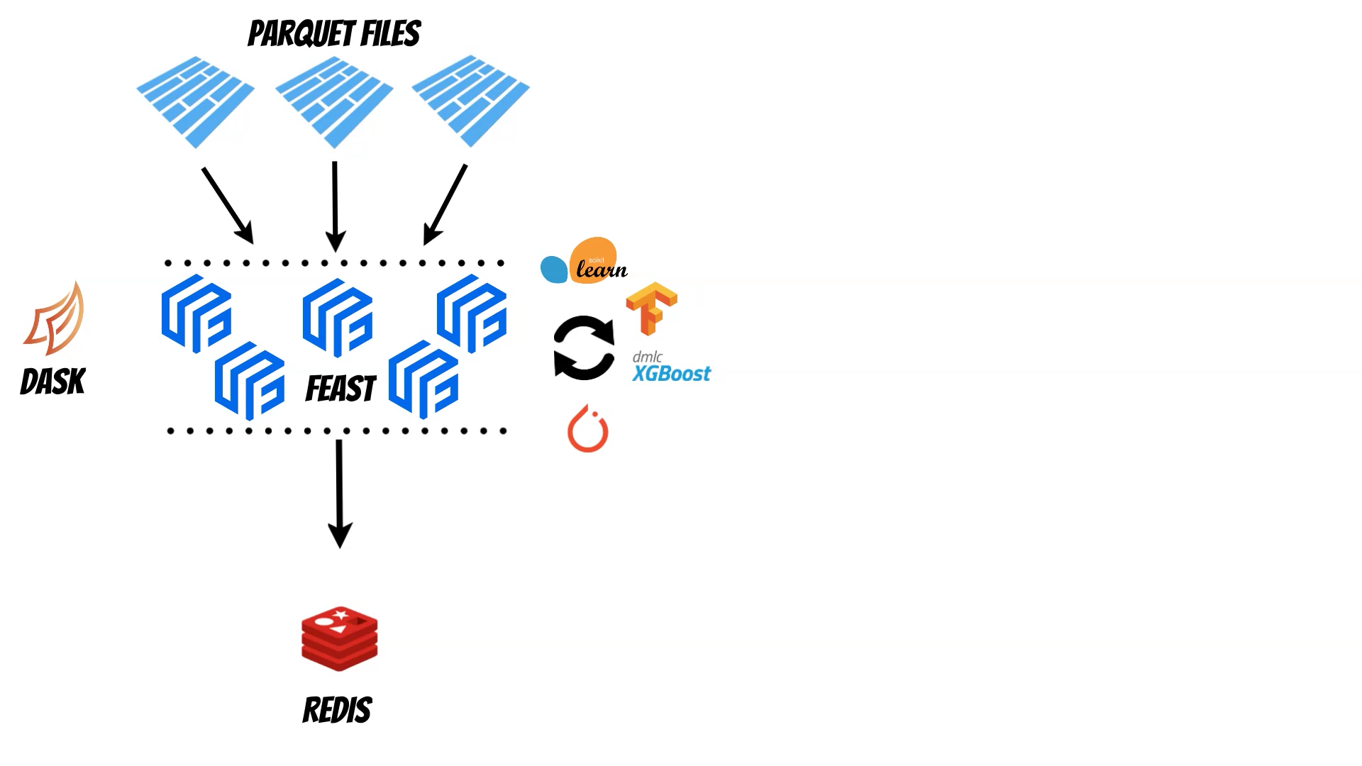
The Feature Store is very important component of the MLops process which helps to manage historical and online features. With the Feast we can for example read historical features from the parquet files and then materialize them to the Redis as a online store.
But what to do if historical data size exceeds our machine capabilities ? The Dask library can help to solve this problem. Using Dask we can distribute the data and calculations across multiple machines. The Dask can be run on the single machine or on the cluster (k8s, yarn, cloud, HPC, SSH, manual setup). We can start with the single machine and then smoothly pass to the cluster if needed. Moreover thanks to the Dask we can read bunch of parquets using path pattern and evaluate distributed training using libraries like scikit-learn or XGBoost
I have prepared ready to use docker image thus you can simply reproduce all steps.
But with the docker you will have the whole environment ready.
In the notebook you will can find all the steps:
Random data generation
I have used numpy and scikit-learn to generate 1M entities end historical data (10 features generated with make_hastie_10_2 function) for 14 days which I save as a parquet file (1.34GB).
Feast configuration and registry
feature_store.yaml - where I use local registry and Sqlite database as a online store.
features.py - with one file source (generate parquet) and features definition.
The create the Feast registry we have to run:
feast apply
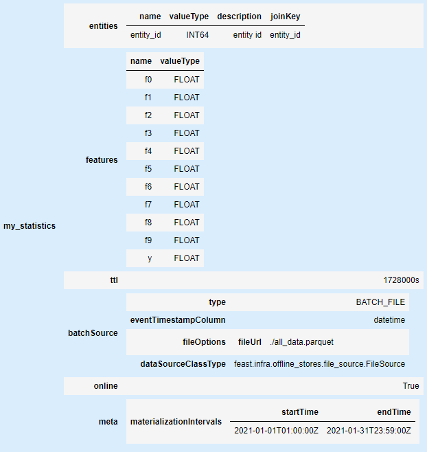
Additionally I have created simple library which helps to inspect feast schema directly in the Jupyter notebook
pip install feast-schema
from feast_schema import FeastSchema

FeastSchema('.').show_schema()
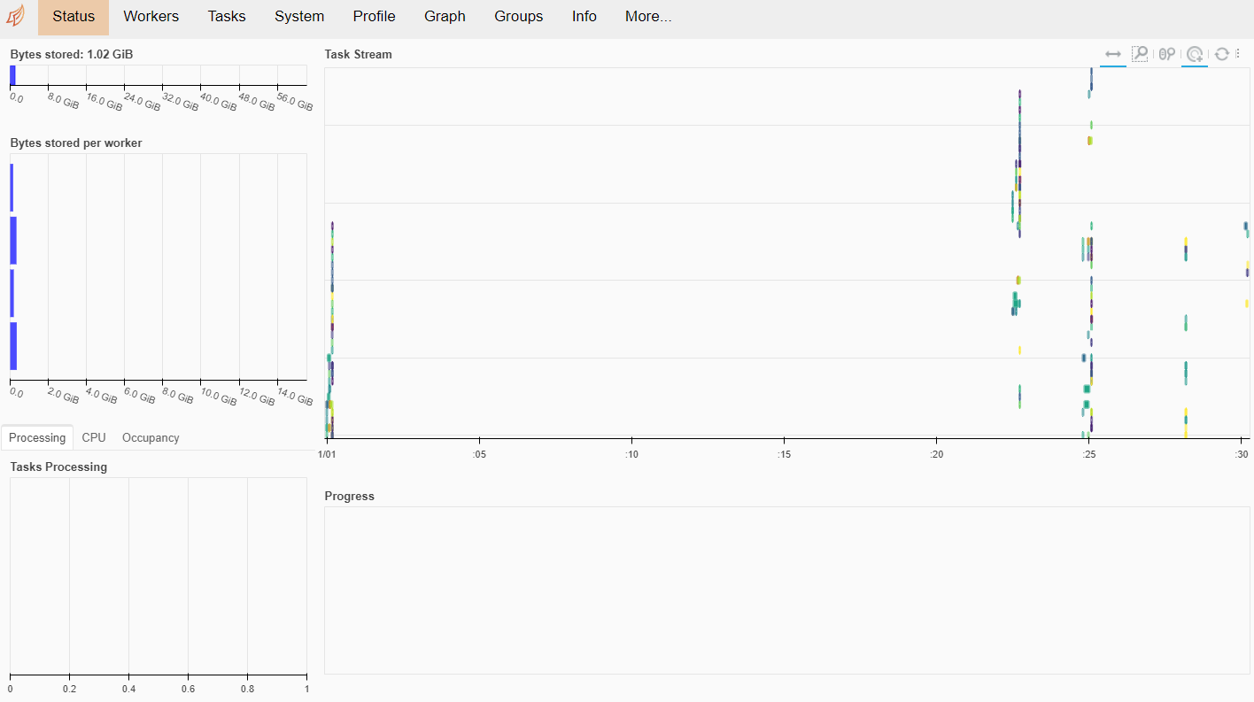
Dask cluster setup
Then I setup simple Dask cluster with scheduler and 4 workers.
Using Dask dataframe we can continue distributed training with the distributed data.
On the other hand if we will use Pandas dataframe the data will be computed to the one node.
To start distributed training with scikit-learn we can use Joblib library with the dask backend:
We use cookies to ensure that we give you the best experience on our website. If you continue to use this site we will assume that you are happy with it.Ok