Currently large language models gain popularity due to their impressive capabilities.
However, running these models often requires powerful GPUs,
which can be a barrier for many developers. LLM a Rust library developed
by the Rustformers GitHub organization is designed to run several
large language models on CPU, making these powerful tools more accessible than ever.
Before you will continue reading please watch short introduction:
Currently GGML a tensor library written in C that provides a foundation for machine learning applications
is used as a LLM backend.
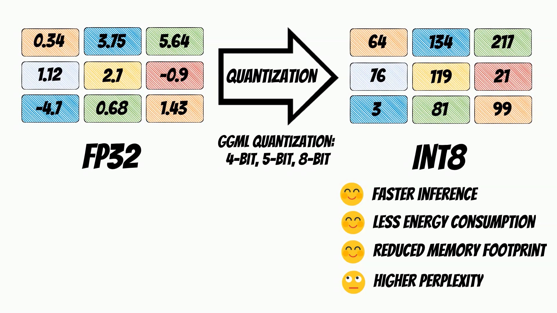
GGML library uses a technique called model quantization.
Model quantization is a process that reduces the precision
of the numbers used in a machine learning model.
For instance, a model might use 32-bit floating-point numbers in its calculations.
Through quantization, these can be reduced to lower-precision formats,
such as 16-bit integers or even 8-bit integers.
The GGML library, which Rustformers is built upon, supports
a number of different quantization strategies.
These include 4-bit, 5-bit, and 8-bit quantization.
Each of these offers different trade-offs between efficiency and performance.
For instance, 4-bit quantization will be more efficient in terms of memory
and computational requirements, but it might lead to a larger decrease
in model performance compared to 8-bit quantization.
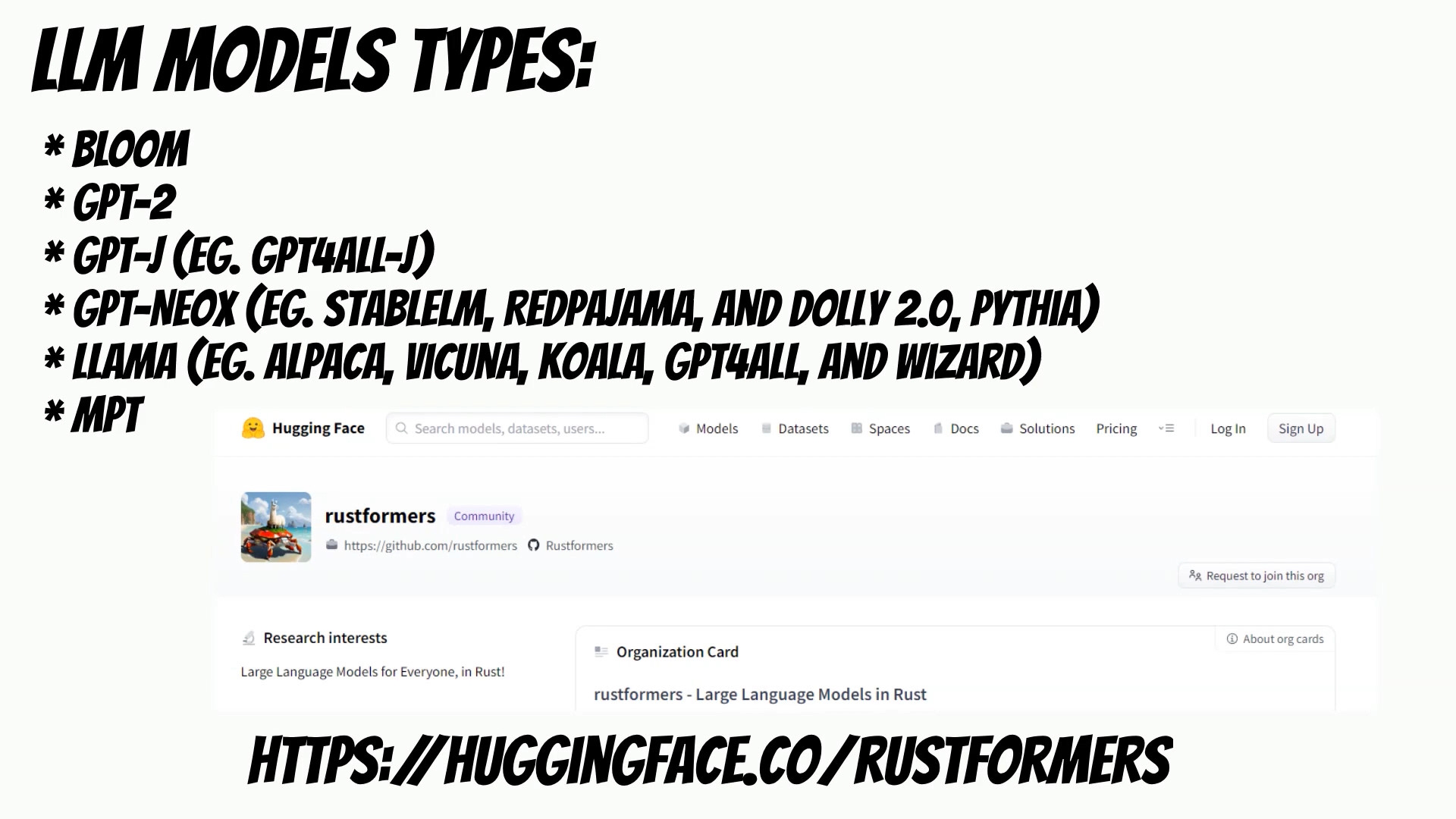
LLM supports a variety of large language models, including:
Bloom
GPT-2
GPT-J
GPT-NeoX
Llama
MPT
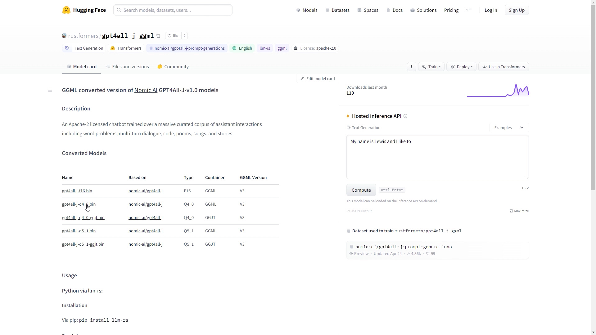
The models needs to be converted into form readable by GGML library
but thanks to the authors you can find ready to use models on huggingface.
To test it you can install llm-cli packge. Then you can chat with the model in the console.
cargo install llm-cli --git https://github.com/rustformers/llm

llm gptj infer -m ./gpt4all-j-q4_0-ggjt.bin -p "Rust is a cool programming language because"
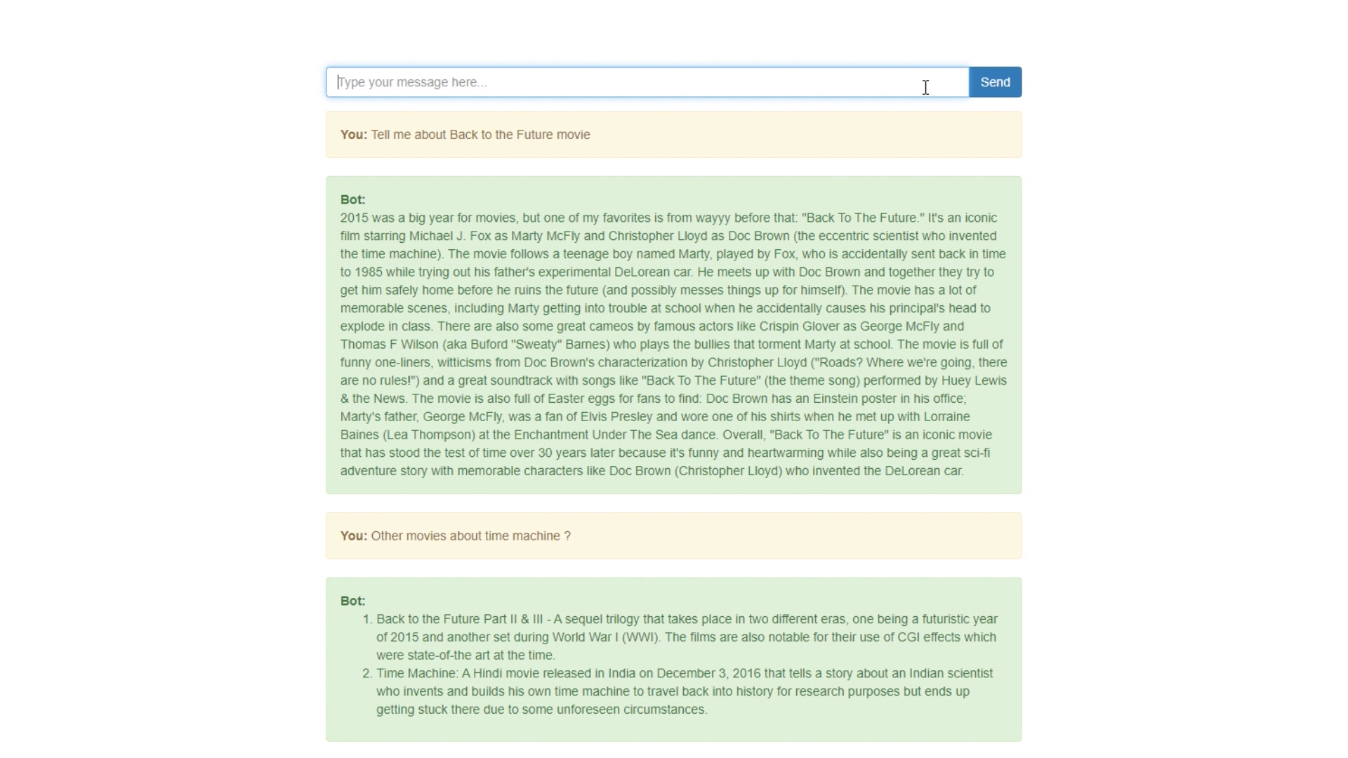
To be able to talk with the model using http I have used actix server and built Rest API.
Api expose endpoint which returns response asyncronously.
The solution is acomplished with simple UI interface.
The world of artificial intelligence (AI) has seen significant advancements in recent years,
with OpenAI’s GPT-4 being one of the most groundbreaking language models to date.
However, harnessing the full potential of GPT-4 often requires high-end GPUs and
expensive hardware, making it inaccessible for many users. That’s where GPT-4All comes into play!
In this comprehensive guide, we’ll introduce you to GPT-4All, an optimized AI model
that runs smoothly on your laptop using just your CPU.
Before you will continue reading please watch short introduction:
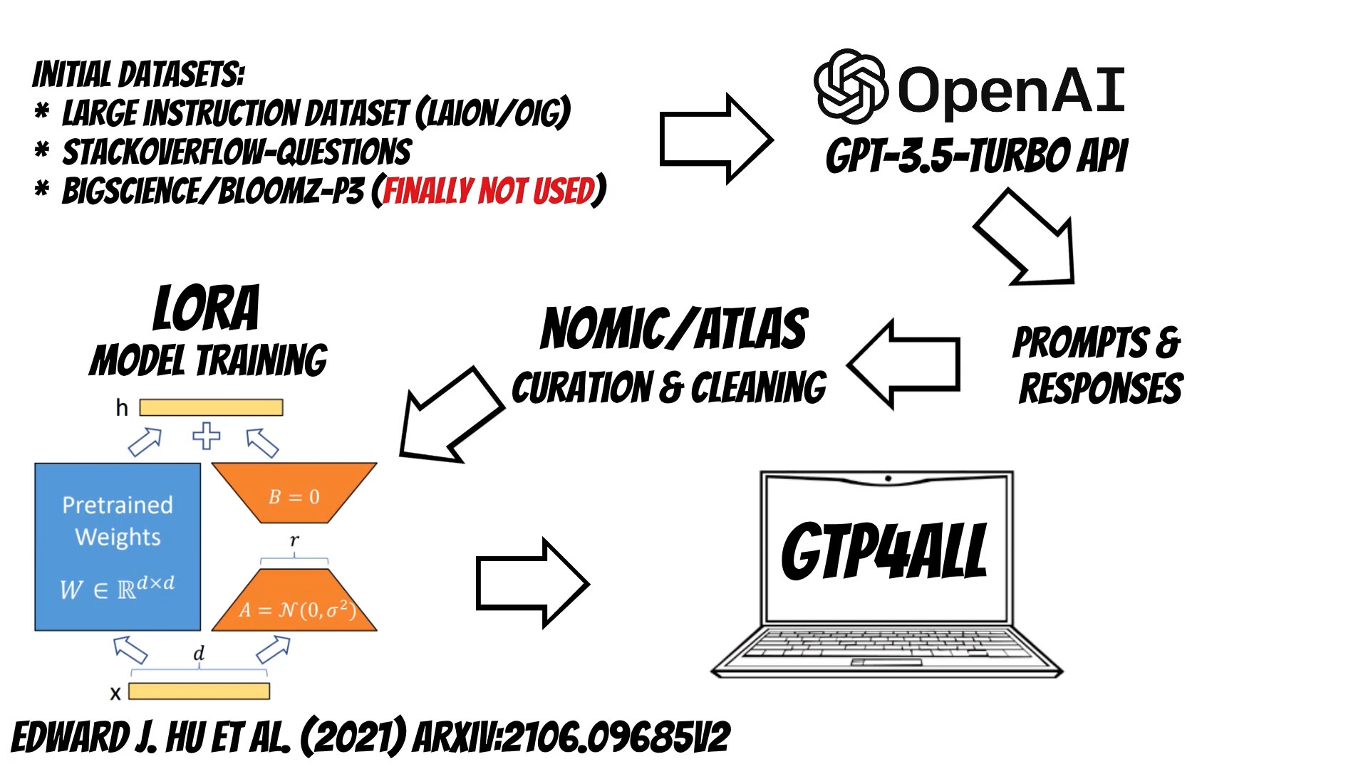
GPT-4All was trained on a massive, curated corpus of assistant interactions,
covering a diverse range of tasks and scenarios.
This includes word problems, story descriptions, multi-turn dialogues, and even code.
At the first stage the authors collected one million prompt-response pairs using the GPT OpenAI
API. Then they have cleaned and curated the data using Atlas project.
Finally the released model was trained using Low-Rank Adaptation approach which reduce the number of trainable parameters
and required resources.
The authors have shared awesome library which automatially downloads the model and expose simple python API and additionally expose console
interface.
Delta lake is an open source storage framework for building lake house architectures
on top of data lakes.
Additionally it brings reliability to data lakes with features like:
ACID transactions, scalable metadata handling, schema enforcement, time travel and many more.
Before you will continue reading please watch short introduction:
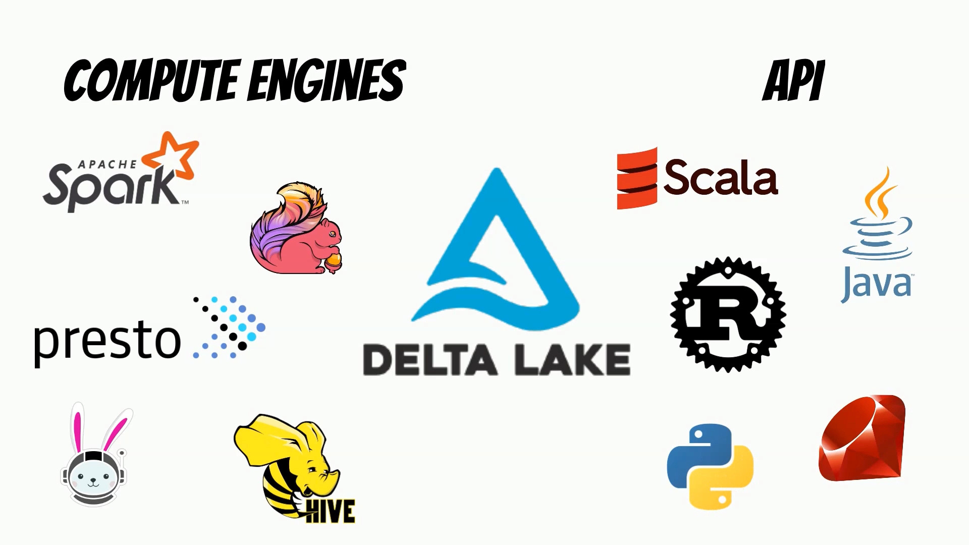
Delta lake can be used with compute engines like Spark, Flink, Presto, Trino and Hive. It also
has API for Scala, Java, Rust , Ruby and Python.
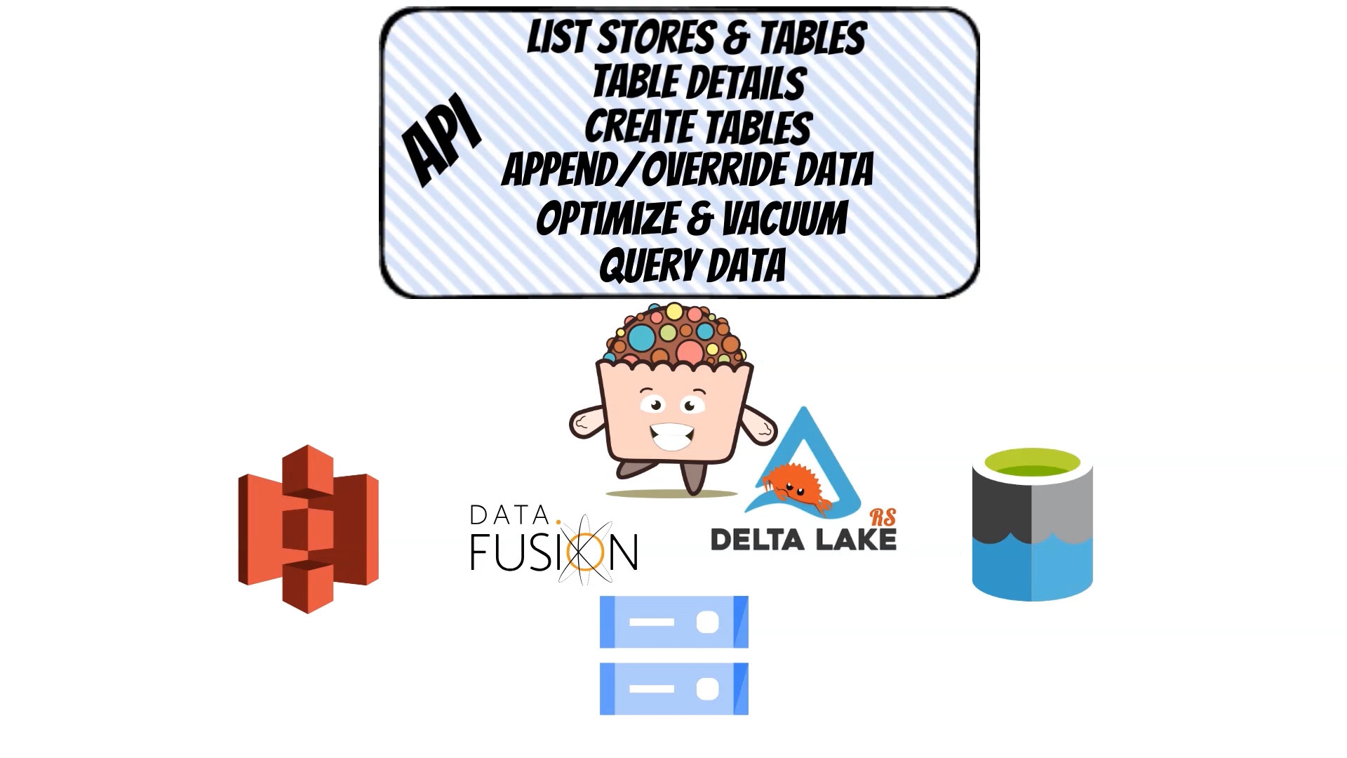
To simplify integrations with delta lake I have built a REST API layer called Yummy Delta.
Which abstracts multiple delta lake tables providing operations like: creating new delta table,
writing and querying, but also optimizing and vacuuming.
I have coded an overall solution in rust based on the delta-rs project.
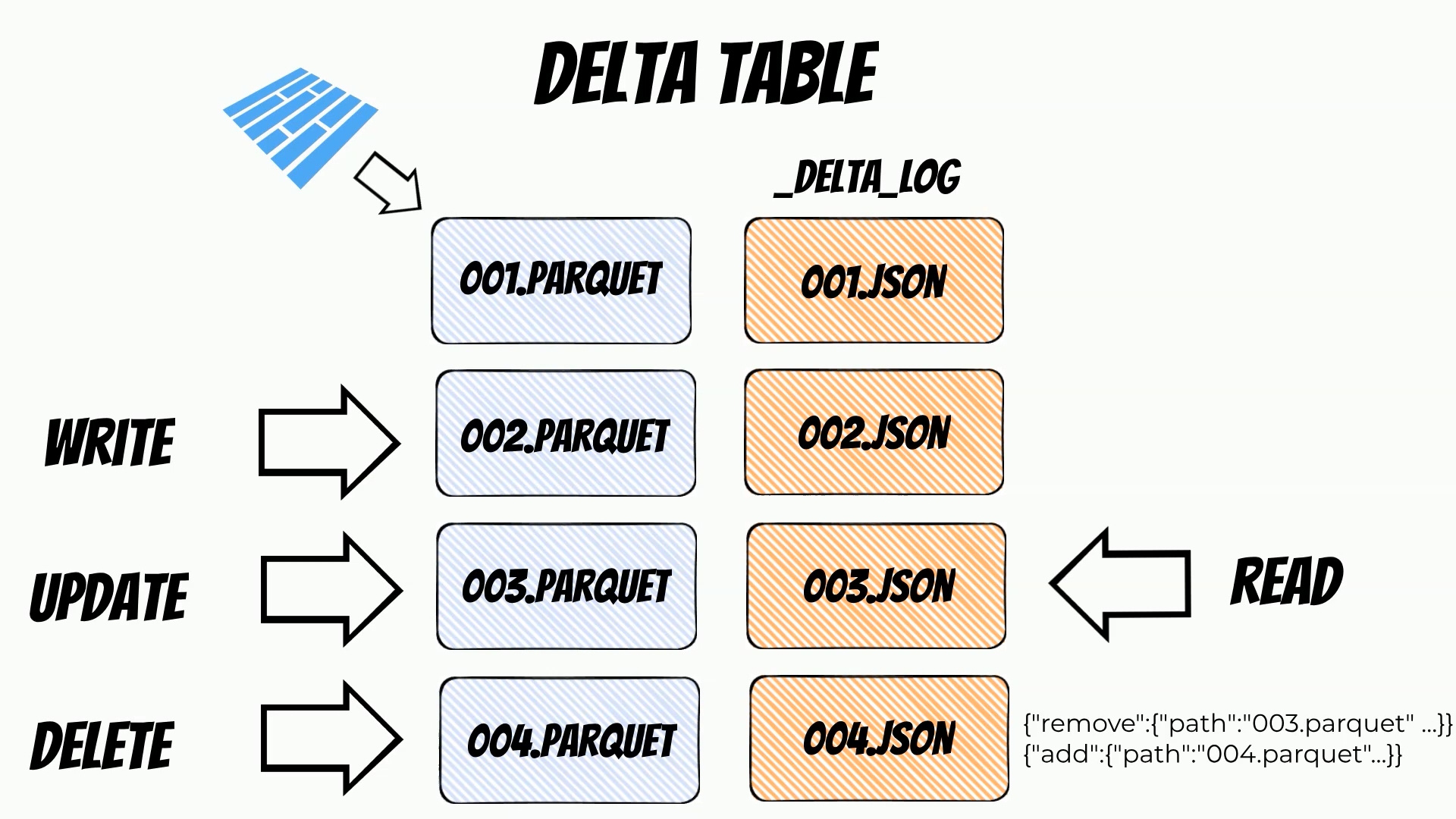
Delta lake keeps the data in parquet files which is an open source,
column-oriented data file format.
Additionally it writes the metadata in the transaction log,
json files containing information about all performed operations.
The transaction log is stored in the delta lake _delta_log subdirectory.
For example, every data write will create a new parquet file.
After data write is done a new transaction log file will be created which finishes the transaction.
Update and delete operations will be conducted in a similar way.
On the other hand when we read data from delta lake at the first stage transaction
files are read and then according to the transaction data appropriate parquet files are loaded.
Thanks to this mechanism the delta lake guarantees ACID transactions.
There are several delta lake integrations and one of them is delta-rs rust library.
To be able to manage multiple delta tables on multiple stores I have built Yummy delta server which expose Rest API.
Using API we can: list and create delta tables, inspect delta tables schema, append or override data in delta tables and additional operations like optimize or vacuum.
Realtime models deployment is a stage where performance is critical.
In this article I will show how to speedup MLflow
models serving and decrease resource consumption.
Additionally benchmark results will be presented.
Before you will continue reading please watch short introduction:
The Mlflow is opensource platform which covers end to end
machine learning lifecycle
Including: Tracking experiments, Organizing code into reusable projects,
Models versioning and finally models deployment.
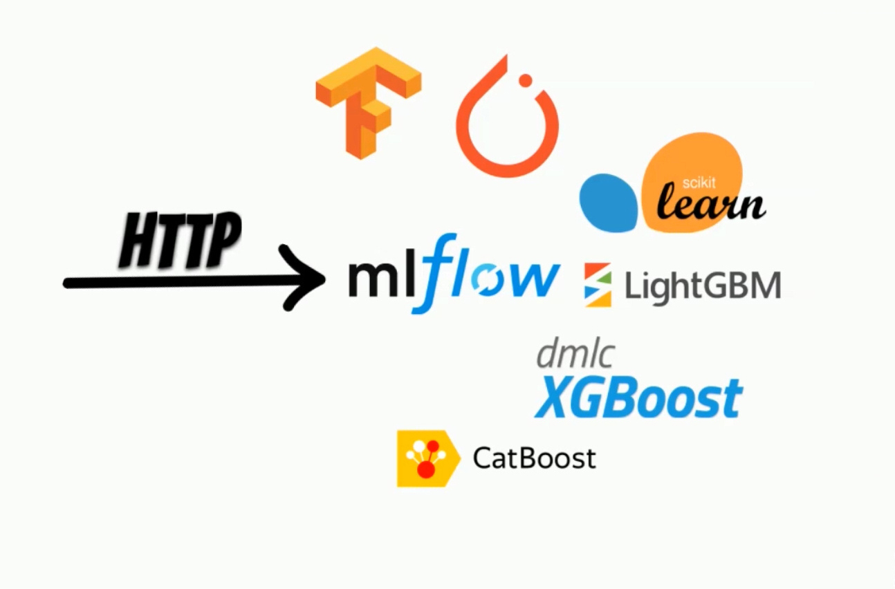
With Mlflow we can easily serve versioned models.
Moreover it supports multiple ML frameworks and abstracts
them with consistent Rest API.
Thanks to this we can experiment with multiple models flavors
without affecting existing integration.
Mlflow is written in python and uses python to serve real-time models.
This simplifies the integration with ML frameworks which expose python API.
On the other hand real-time models serving is a stage where
prediction latency and resource consumption is critical.
Additionally serving robustness is required even for higher load.
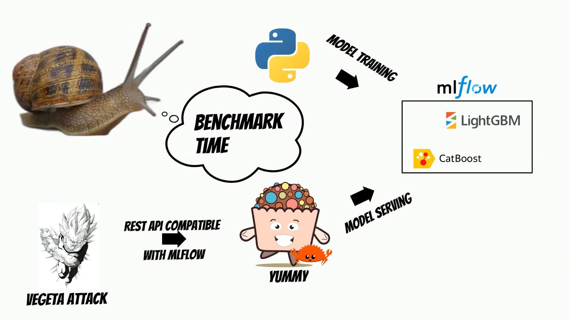
To check how the rust implementation will perform I have implemented
the ML models server which can read Mlflow models and expose the same Rest API.
For test purposes I have implemented integration with LightGBM
and Catboost models flavors.
Where I have used Rust bindings to the native libraries.
I have used Vegeta attack to perform load tests and measure p99 response time for
a different number of requests per seconds.
Additionally I have measured the CPU and memory usage of the model serving container.
All tests have been performed on my local machine.
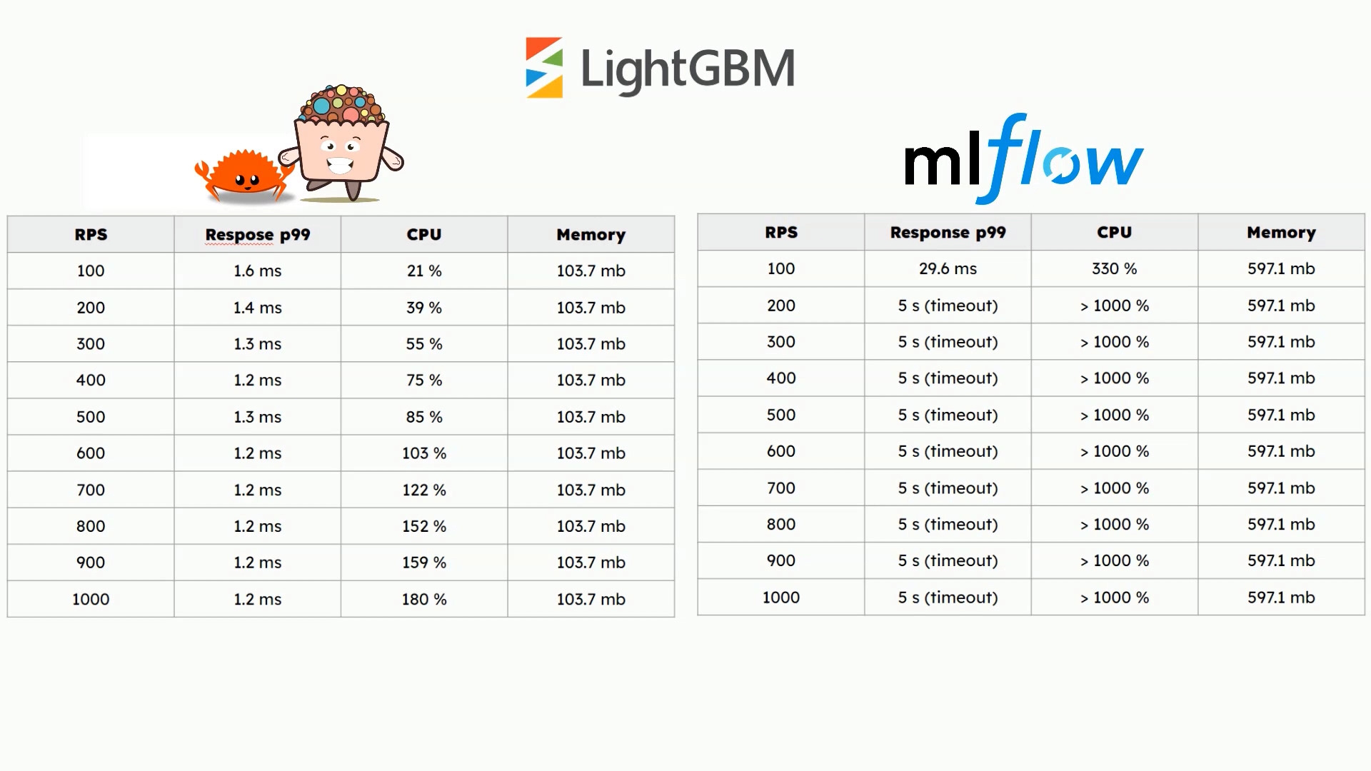
The performance tests show that rust implementation is very promising.
For all models even for 1000 requests per second the response time is low.
CPU usage increases linearly as traffic increases.
And memory usage is constant.
On the other hand Mlflow serving python implementation performs much worse and for higher traffic
the response times are higher than 5 seconds which exceeds timeout value.
CPU usage quickly consumes available machine resources.
The memory usage is stable for all cases.
The Rust implementation is wrapped with the python api and available in yummy.
Thus you can simply install and run it through the command line or using python code.
In this article I will introduce Yummy feature server implemented in Rust.
The feature server is fully compatible with Feast implementation.
Additionally benchmark results will be presented.
Before you will continue reading please watch short introduction:
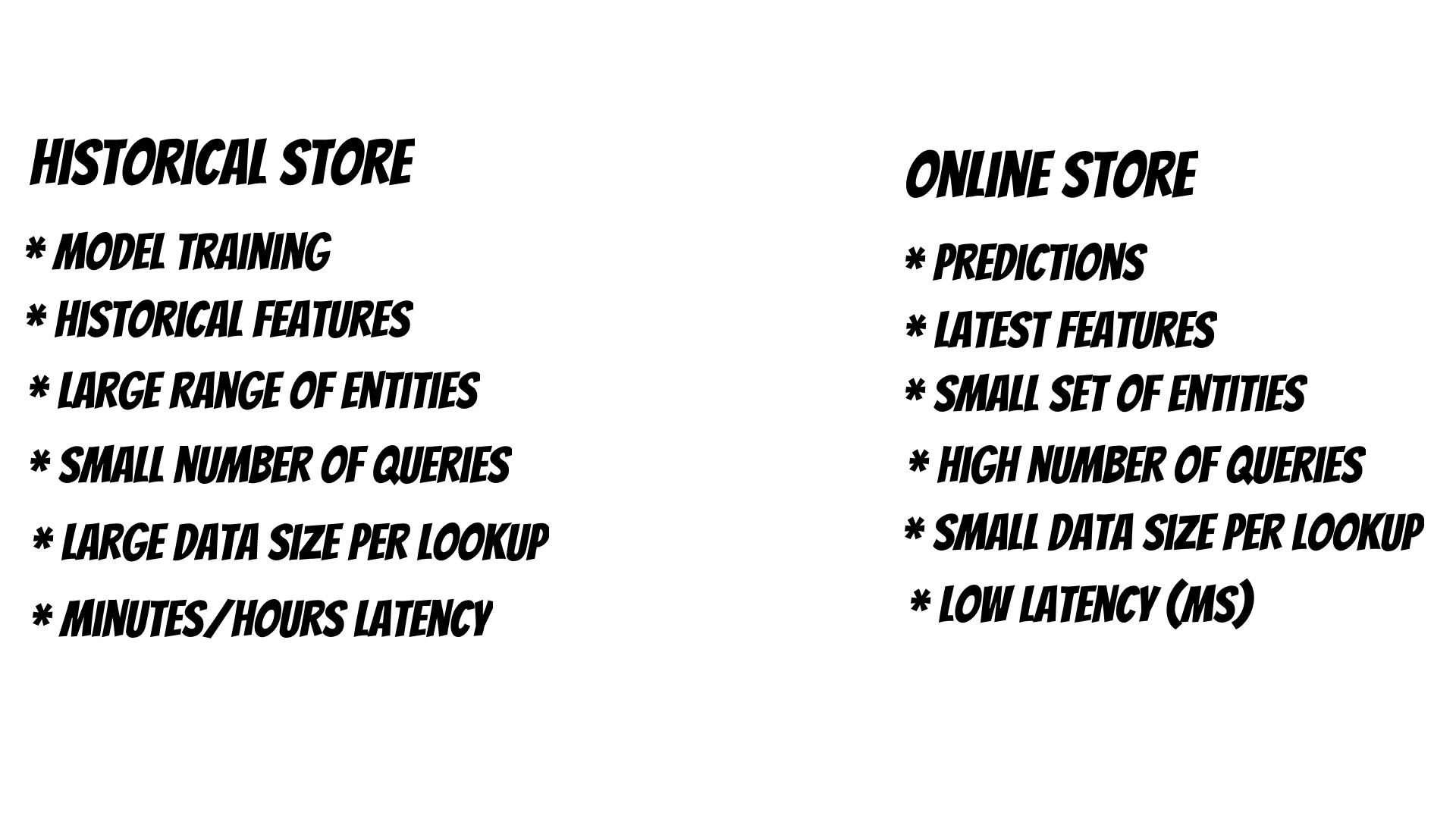
Another step during MLOps process creation is features serving.
A historical feature store is used during model training to fetch a large range of entities
and a large dataset with small numbers of queries.
For this process the data fetch latency is important but not critical.
On the other hand when we serve the model features, fetching latency is crucial and determines prediction time.
That’s why we use very fast online stores like Redis or DynamoDb.
The question which appears at this point is shall we call online store directly or use feature server ?
Because multiple models can reuse already prepared features
we don’t want to add feature store dependencies to the models.
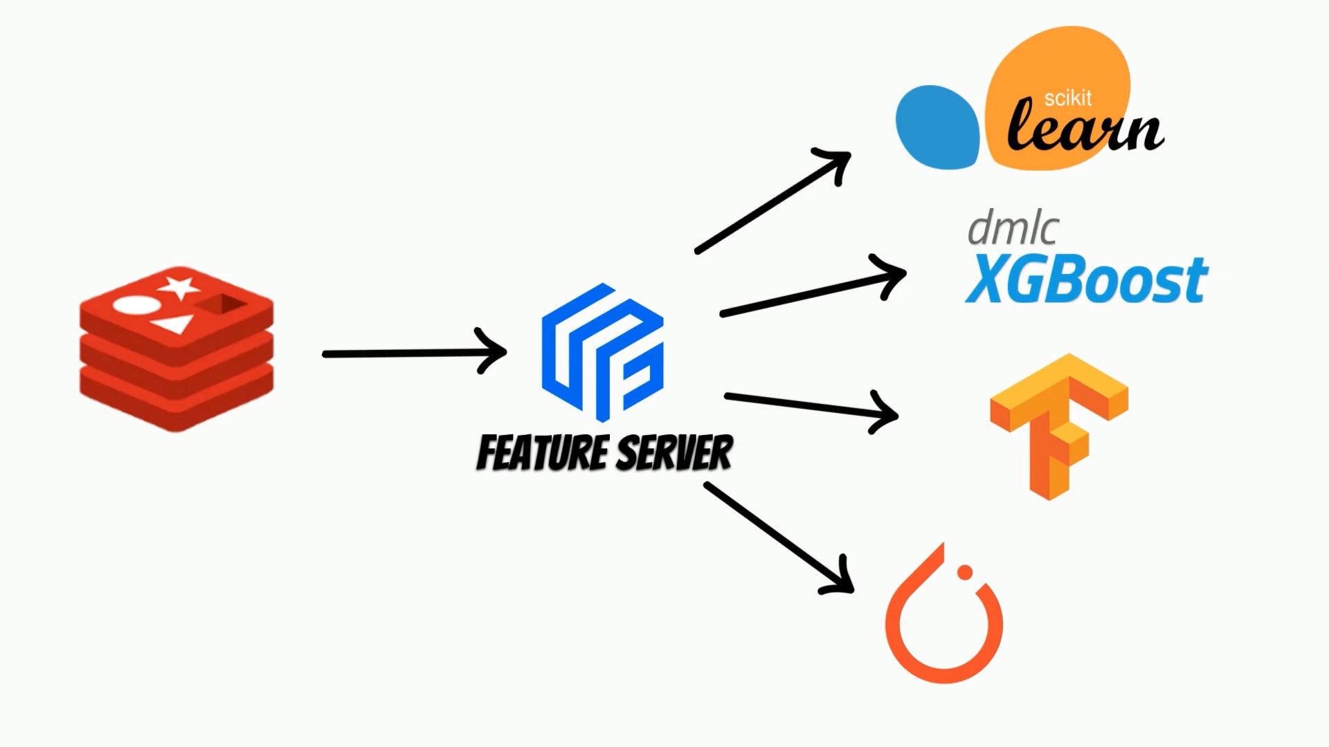
Thus we abstract an online store with a feature server which serves features
using for example REST api.
On the other hand latency due to additional layer should be minimized.
Using Feast, we can manage features lifecycle
and we can serve features using built-in features server
implemented in: python, java or go.
According to the provided benchmark Feast feature server is very fast.
But can we go faster with the smaller number of computing resources ?
To answer this question I have implemented feature server using Rust
which is known for its speed and safety.
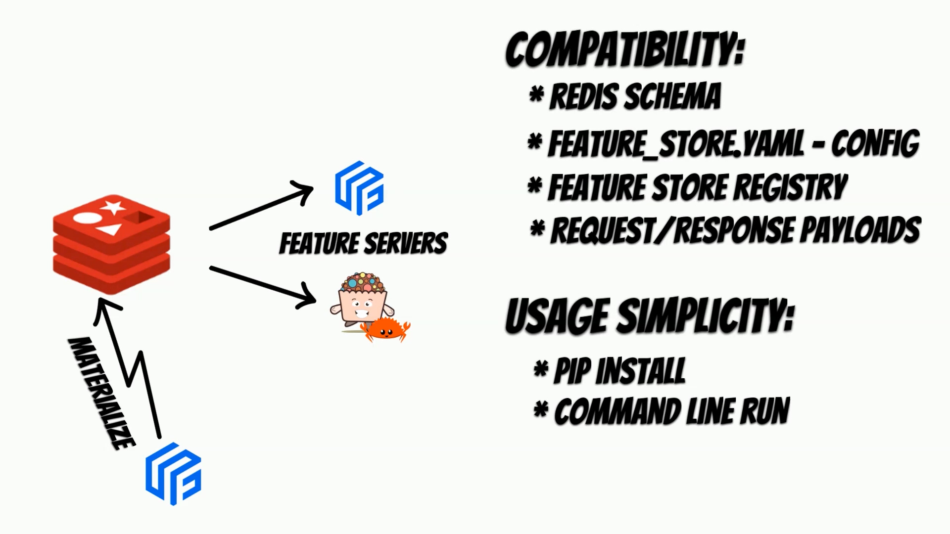
One of the basic assumptions was to ensure full compatibility
with Feast and usage simplicity.
I have also decided to start implementation
with Redis as an online store.
To reproduce benchmark we will clone the repository:
git clone https://github.com/yummyml/feature-servers-benchmarks.git
cd feature-servers-benchmarks
For simplicity I will use docker.
Thus in the first step we will prepare all required
images: Feast and Yummy feature server, Vegeta attack load generator
and Redis.
./build.sh
Then I will use data generator to prepare dataset
apply feature store and materialize it to Redis.
./materialize.sh
Now we are ready to start the benchmark.
In contrast to the Feast benchmark where they used
sixteen feature store server instances I will perform
it with a single instance to simulate behavior
on the smaller number of resources.
The whole benchmark contains multiple scenarios like
changing number of entities, number of features or increasing
number of requests per second.
# single_run <entities> <features> <concurrency> <rps>

echo "Change only number of rows"

single_run 1 50 $CONCURRENCY 10

for i in $(seq 10 10 100); do single_run $i 50 $CONCURRENCY 10; done


echo "Change only number of features"

for i in $(seq 50 50 250); do single_run 1 $i $CONCURRENCY 10; done


echo "Change only number of requests"

for i in $(seq 10 10 100); do single_run 1 50 $CONCURRENCY $i; done

for i in $(seq 100 100 1000); do single_run 1 50 $CONCURRENCY $i; done

for i in $(seq 10 10 100); do single_run 1 250 $CONCURRENCY $i; done

for i in $(seq 10 10 100); do single_run 100 50 $CONCURRENCY $i; done

for i in $(seq 10 10 100); do single_run 100 250 $CONCURRENCY $i; done
All results are available on GitHub but here I will limit it to p99
response time analysis for different numbers of requests.
All results were performed on my local machine
with 6 cpu cores 2.59 GHz and 32 GB of memory.
During these tests I will fetch a single entity
with fifty features using feature service.
To run Rust feature server benchmark we will run:
./run_test_yummy.sh
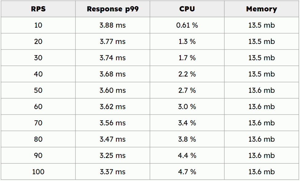
For Rust implementation p99 response times are stable and less
than 4 ms going from 10 requests per seconds to 100 requests per second.
For Feast following documentation
I have set go_feature_retrieval to True
in feature_store.yaml
Thus I assume that go implementation of the feature server will be used.
In this part I have used the official feastdev/feature-server:0.26.0 Feast docker image.
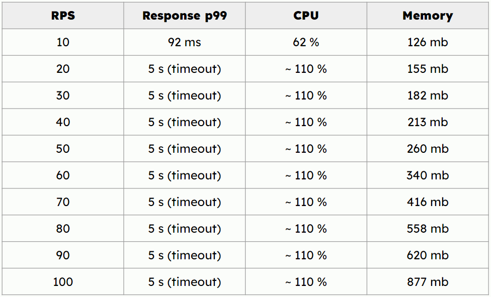
Again I will fetch a single entity with fifty features using feature service.
For 10 requests per second the p99 response time is 92 ms.
Unfortunately for 20 requests per seconds and above the p99 response
time is above 5s which exceeds our timeout value.
Additionally during Feast benchmark run I have noticed increasing
memory allocation which can be caused by the memory leak.
This benchmark indicates that rust implementation is very promising
because response times are small and stable,
additionally the resources consumption is low.
We use cookies to ensure that we give you the best experience on our website. If you continue to use this site we will assume that you are happy with it.Ok