Today I’m very happy to finally release my open source project DeepMicroscopy.
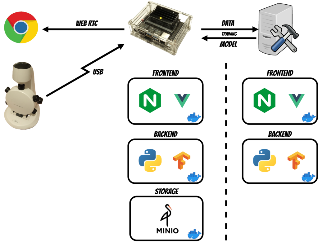
In this project I have created the platform where you can capture the images from the microscope, annotate, train the Tensorflow model and finally observe real time object detection.
The project is configured on the Jetson Nano device thus it can work with compact and portable solutions.
Backend - Python application which handles the training logic
2. Platform functionalities
The most of platform’s functionality is installed on the Jetson Nano. Because the Jetson Nano compute capabilities are insufficient for model training purposes I have decided to split this part into three stages which I will describe in the training paragraph.
Projects management
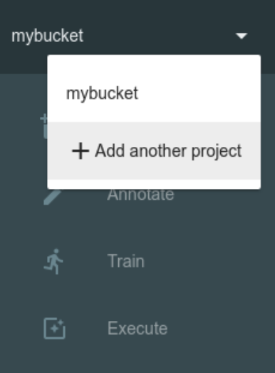
In the Deep Microscopy you can create multiple projects where you annotate and recognize different objects.
You can create and switch projects in the top left menu. Each project data is kept in the separate bucket in the minio storage.
Images Capture
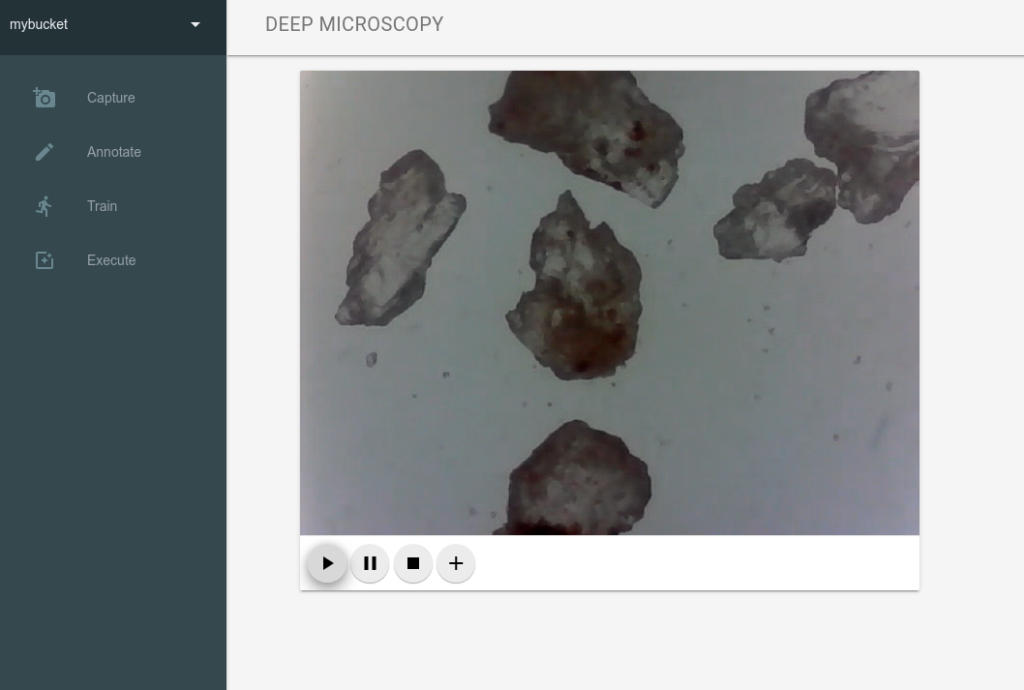
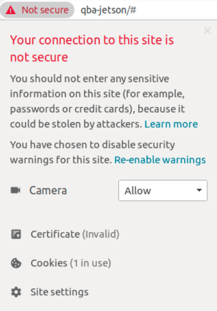
When you open the Capture panel in the web application and click Play ▶ button the WebRTC socket between browser and backend is created (I have used the aiortc python library). To make it working in the Chrome browser we need two things:
use TLS for web application - the self signed certificate is already configured in the nginx
allow Camera to be used for the application - you have to set it in the browser
Now we can stream the image from camera to the browser (I have used OpenCV library to fetch the image from microscope through usb).
When we decide to capture specific frame and click Plus ✚ button the backend saves the current frame into project bucket of minio storage.
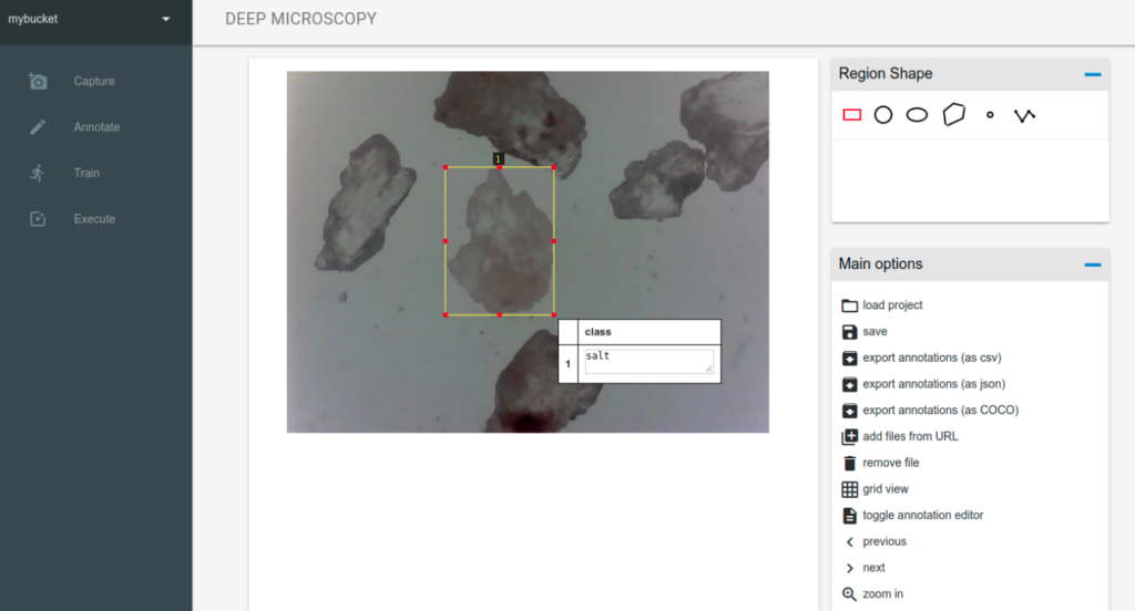
Annotation
The annotation engine is based on the Via Image Annotator. Here you can see all images you have captured for specific project. There are a lot of features eg. switching between images (left/right arrow), zoom in/out (+/-) and of course annotation tools with different shapes (currently the training algorithm expects the rectangles) and attributes (by default the class attribute is added which is also expected by the training algorithm).
This is rather painstaking and manual task thus when you will finish remember to save the annotations by clicking save button (currently there is no auto save). When you save the project the project file (with the via schema) is saved in the project bucket.
Training
When we finish image annotation we can start model training. As mentioned before it is split into three stages.
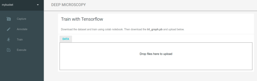
Data package
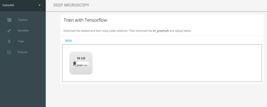
At the beginning we have to prepare data package (which contains captured images and our annotations) by clicking the DATA button.
Training server
Then we drag and drop the data package to the application placed on machine with higher compute capabilities.
After upload the training server automatically extracts the data package, splits into train/test data and starts training.
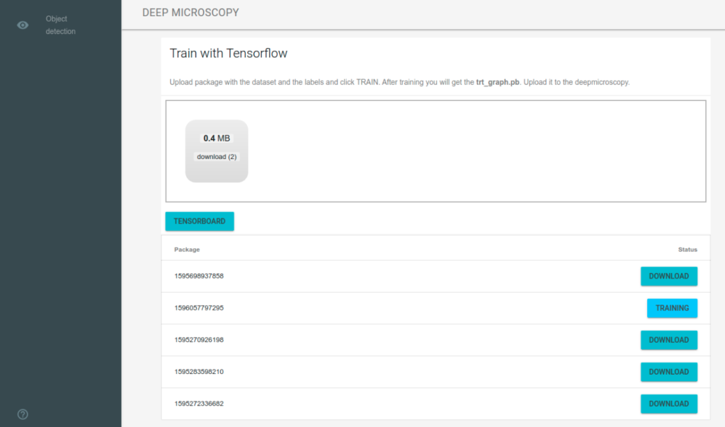
Currently I have used the MobileNet V2 model architecture and I base on the pretrained tensorflow model.
When the training is finished the model is exported using TensorRT which optimizes the model inference performance especially on NVIDIA devices like Jetson Nano.
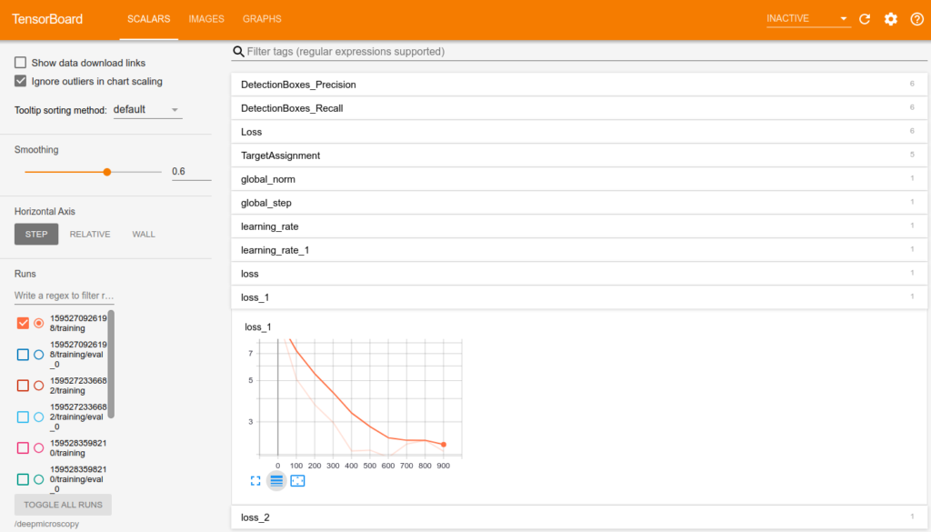
During and after training you can inspect all models using builtin tensorboard.
The web application periodically check training state and when the training is finished we can download the model.
Uploading model
Finally we upload the TensorRT model back to the Jetson Nano device. The model is saved into selected project bucket thus you can use multiple models for each project.
Object detection
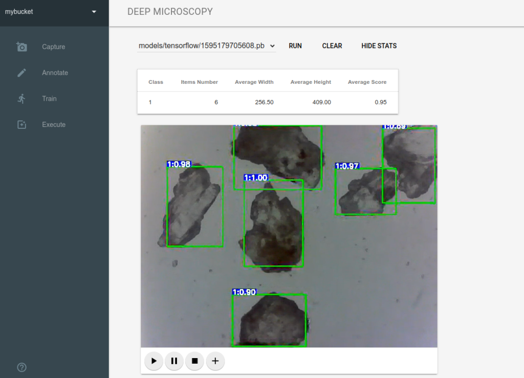
On the Execute panel we can choose model from the drop down list (where we have list of models uploaded for selected project) and load the model clicking RUN (typically it take same time to load the model). When we click Play ▶ button the application shows real time object detection. If we want to change the model we can click CLEAR and then choose and RUN another model.
Additionally we can fetch additional detection statistics which are sent using Web Socket. Currently the number of detected items and average width, height, score are returned.
Jupyter Notebook is one of the most useful tool for data exploration, machine learning and fast prototyping. There are many plugins and projects which make it even more powerful:
One of my favorite text editor is vim. It is lightweight, fast and with appropriate plugins it can be used as a IDE.
Using Dockerfile you can build jupyter environment with fully equipped vim:
FROM continuumio/miniconda3
RUN apt update && apt install curl git cmake ack g++ python3-dev vim-youcompleteme tmux -yq
RUN sh -c "$(curl -fsSL https://raw.githubusercontent.com/qooba/vim-python-ide/master/setup.sh)"
RUN conda install xeus-python jupyterlab jupyterlab-git -c conda-forge
RUN jupyter labextension install @jupyterlab/debugger @jupyterlab/git
RUN pip install nbdev
RUN echo "alias ls='ls --color=auto'" >> /root/.bashrc
CMD bin/bash
IoT and AI are the hottest topics nowadays which can meet on Jetson Nano device.
In this article I’d like to show how to use FastAI library, which is built on the top of the PyTorch on Jetson Nano. Additionally I will show how to optimize the FastAI model for the usage with TensorRT.
Although the Jetson Nano is equipped with the GPU it should be used as a inference device rather than for training purposes. Thus I will use another PC with the GTX 1050 Ti for the training.
Docker gives flexibility when you want to try different libraries thus I will use the image which contains the complete environment.
Training environment Dockerfile:
FROM nvcr.io/nvidia/tensorrt:20.01-py3
WORKDIR /
RUN apt-get update && apt-get -yq install python3-pil
RUN pip3 install jupyterlab torch torchvision
RUN pip3 install fastai
RUN DEBIAN_FRONTEND=noninteractive && apt update && apt install curl git cmake ack g++ tmux -yq
RUN pip3 install ipywidgets && jupyter nbextension enable --py widgetsnbextension
CMD ["sh","-c", "jupyter lab --notebook-dir=/opt/notebooks --ip='0.0.0.0' --port=8888 --no-browser --allow-root --NotebookApp.password='' --NotebookApp.token=''"]
To use GPU additional nvidia drivers (included in the NVIDIA CUDA Toolkit) are needed.
If you don’t want to build your image simply run:
docker run --gpus all --name jupyter -d --rm -p 8888:8888 -v $(pwd)/docker/gpu/notebooks:/opt/notebooks qooba/fastai:1.0.60-gpu
Now you can use pets.ipynb notebook (the code is taken from lesson 1 FastAI course) to train and export pets classification model.
from fastai.vision import *
from fastai.metrics import error_rate

# download dataset
path = untar_data(URLs.PETS)
path_anno = path/'annotations'
path_img = path/'images'
fnames = get_image_files(path_img)

# prepare data
np.random.seed(2)
pat = r'/([^/]+)_\d+.jpg$'
bs = 16
data = ImageDataBunch.from_name_re(path_img, fnames, pat, ds_tfms=get_transforms(), size=224, bs=bs).normalize(imagenet_stats)

# prepare model learner
learn = cnn_learner(data, models.resnet34, metrics=error_rate)

# train
learn.fit_one_cycle(4)

# export
learn.export('/opt/notebooks/export.pkl')
Finally you get pickled pets model (export.pkl).
2. Inference (Jetson Nano)
The Jetson Nano device with Jetson Nano Developer Kit already comes with the docker thus I will use it to setup the inference environment.
With big pleasure I would like to invite you to join Azuronet - .NET & Azure Meetup #2 in Warsaw, where I will talk (in polish) about Milla project and give you some insights into the world of chatbots and intelligent assistants.
I am pleased to hear that the first Polish banking chatbot with which you can make a transfer was awarded in a competition organized by a Gazeta Bankowa. With Milla you can talk in the Bank Millennium mobile application. Currently, Milla can speak (text to speech), listen (automatic speak recognition) and understand what you write to her (intent detection with slot filling).
This is not a sponsored post :) but I’ve been developing Milla for the few months and I’m really happy that I had opportunity to do this.
We use cookies to ensure that we give you the best experience on our website. If you continue to use this site we will assume that you are happy with it.Ok